Thermal and hyperspectral sensing

Two questions from the board needed more than the reflective bands of Sentinel-2. The first was how much water the crops were actually using, compared with what the district delivered; the second was whether water was seeping through the new embankments into the fields below, where two farmers had reported soft ground. Both pointed to thermal sensing: an evaporating surface is cooler than a dry one, so temperature carries information about water. A third, longer-term question came from the agronomist on the board, who had read that hyperspectral satellites could detect nutrient deficiencies and asked whether the district should be using them. This lesson covers thermal infrared remote sensing, from radiance to land surface temperature and evapotranspiration, and hyperspectral imaging, its data, its analysis by spectral unmixing and its uses.

Thermal radiance and brightness temperature

In the thermal window between about 8 and 14 µm, the radiance leaving the surface is almost entirely emitted, as Lesson 1 showed. A thermal sensor records at-sensor radiance, calibrated from digital numbers with a gain and offset like the reflective bands. Inverting Planck's law for a blackbody gives the brightness temperature, the temperature a blackbody would need to produce the observed radiance. For a narrow band, the inversion is written with two calibration constants supplied in the metadata:

For band 10 of Landsat's Thermal Infrared Sensor the constants are about \(K_1 = 774.89\) W m⁻² sr⁻¹ µm⁻¹ and \(K_2 = 1321.08\) K. Brightness temperature is not yet surface temperature. Three corrections remain: for emissivity, because real surfaces emit less than a blackbody; for the atmosphere, which absorbs part of the surface emission and adds its own; and for reflected downwelling sky radiance, which is small but not negligible for low-emissivity surfaces.

Land surface temperature

The emissivity correction can be approximated, for a single band and ignoring the atmosphere, by

An error of 0.01 in emissivity produces an error of roughly 0.5 to 0.7 K in surface temperature at 10 µm, so emissivity matters. It is estimated from land cover classes, from NDVI through the fraction of vegetation cover, or, for sensors with several thermal bands, by temperature-emissivity separation algorithms. Atmospheric correction uses radiative transfer models with water vapor profiles; the split-window method uses two thermal bands, such as Landsat's bands 10 and 11 near 10.9 and 12.0 µm, whose different water vapor absorption allows the atmospheric effect to be estimated. Standard Level-2 surface temperature products apply these corrections, with typical accuracies of about 1 to 2 K over vegetated land in clear conditions, poorer in humid air and over surfaces with uncertain emissivity.

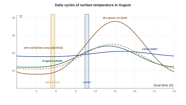
Surface temperature is the skin temperature of the top fraction of a millimeter of whatever the sensor sees: leaves, soil, roof or water. It differs from air temperature, often by several degrees and by tens of degrees for dry soil and pavement in afternoon sun. It changes quickly through the day, rising from a minimum near dawn to a maximum in early afternoon, with a range that depends on the thermal inertia of the surface, its ability to resist temperature change. Water has high thermal inertia and changes little; dry soil and gravel have low thermal inertia and change greatly. Moist soil has higher thermal inertia than dry soil and also loses heat by evaporation, so it is cooler by day and warmer by night than dry soil, a contrast greatest near dawn for some surfaces and near midday for others.

import math
# Landsat TIRS band 10 style calibration constants (from the scene metadata)
ML, AL = 3.342e-4, 0.1           # radiance = ML * DN + AL, W m-2 sr-1 um-1
K1, K2 = 774.8853, 1321.0789     # thermal constants for band 10
lam = 10.895e-6                  # effective wavelength, m
def bt(L): return K2 / math.log(K1 / L + 1.0)
pix = {"canal water": 24120, "seepage strip below the bank": 24860, "irrigated alfalfa": 25010,
       "dry grass on the bank": 28940, "gravel road": 30310}
print("pixel                           DN    radiance  brightness T   LST (emissivity)")
rho = 1.438e-2                   # h c / k, m K
eps = {"canal water": 0.99, "seepage strip below the bank": 0.98, "irrigated alfalfa": 0.985,
       "dry grass on the bank": 0.96, "gravel road": 0.95}
for k, dn in pix.items():
    L = ML * dn + AL
    T = bt(L)
    lst = T / (1 + (lam * T / rho) * math.log(eps[k]))
    print(f"{k:30s} {dn:6d}  {L:7.3f}   {T - 273.15:6.2f} C    {lst - 273.15:6.2f} C ({eps[k]})")

# Seepage screening: flag pixels on the downslope side that are cooler than the dry-bank average
bank = [31.8, 32.4, 31.1, 30.9, 24.6, 23.9, 31.5, 32.0, 25.2, 31.7, 32.6, 31.3]   # LST along 12 bank segments, C
dry = sorted(bank)[len(bank) // 2]
print(f"\nmedian bank LST {dry:.1f} C")
for i, t in enumerate(bank):
    if dry - t > 4.0: print(f"  segment {i + 1:2d}: {t:.1f} C, {dry - t:.1f} C cooler -> inspect for seepage")

# Linear spectral unmixing of one 30 m hyperspectral pixel into three endmembers (6 bands shown)
em = {"alfalfa": [0.03, 0.07, 0.035, 0.48, 0.20, 0.09],
      "bare soil": [0.10, 0.14, 0.18, 0.23, 0.30, 0.25],
      "water": [0.06, 0.07, 0.04, 0.02, 0.008, 0.005]}
x = [0.058, 0.093, 0.093, 0.284, 0.202, 0.141]
names = list(em); A = [[em[k][b] for k in names] for b in range(6)]
# least squares with the sum-to-one constraint added as a heavily weighted extra row
w = 100.0
A2 = A + [[w, w, w]]; x2 = x + [w]
AtA = [[sum(A2[r][i] * A2[r][j] for r in range(7)) for j in range(3)] for i in range(3)]
Atx = [sum(A2[r][i] * x2[r] for r in range(7)) for i in range(3)]
# solve the 3 x 3 system by Cramer's rule
def det(M): return (M[0][0] * (M[1][1] * M[2][2] - M[1][2] * M[2][1]) - M[0][1] * (M[1][0] * M[2][2] - M[1][2] * M[2][0]) + M[0][2] * (M[1][0] * M[2][1] - M[1][1] * M[2][0]))
D = det(AtA); f = []
for j in range(3):
    M = [row[:] for row in AtA]
    for i in range(3): M[i][j] = Atx[i]
    f.append(det(M) / D)
print("\nfractions:", ", ".join(f"{k} {v:.3f}" for k, v in zip(names, f)))
resid = [x[b] - sum(A[b][j] * f[j] for j in range(3)) for b in range(6)]
print("RMS residual reflectance", f"{math.sqrt(sum(r * r for r in resid) / 6):.4f}")

pixel                           DN    radiance  brightness T   LST (emissivity)
canal water                     24120    8.161    16.32 C     16.96 C (0.99)
seepage strip below the bank    24860    8.408    18.20 C     19.51 C (0.98)
irrigated alfalfa               25010    8.458    18.58 C     19.56 C (0.985)
dry grass on the bank           28940    9.772    28.07 C     30.90 C (0.96)
gravel road                     30310   10.230    31.21 C     34.85 C (0.95)

median bank LST 31.5 C
  segment  5: 24.6 C, 6.9 C cooler -> inspect for seepage
  segment  6: 23.9 C, 7.6 C cooler -> inspect for seepage
  segment  9: 25.2 C, 6.3 C cooler -> inspect for seepage

fractions: alfalfa 0.393, bare soil 0.404, water 0.204
RMS residual reflectance 0.0038

The code shows how the corrections work and how much they matter. The dry grass on the bank has a brightness temperature of 28.1 °C but, with an emissivity of 0.96, a surface temperature of 30.9 °C; the canal water, with an emissivity of 0.99, changes by less than a degree. The screening step compares each of twelve segments of the embankment with the median of all segments and flags those more than 4 °C cooler: segments 5, 6 and 9, which are 6 to 8 °C cooler than the dry bank, are candidates for seepage.

Thermal sensing of water use and seepage

Evapotranspiration (ET), the combined evaporation from soil and transpiration from plants, consumes energy: vaporizing water takes about 2.45 MJ per kilogram. A well-watered crop transpires freely and stays cool, while a stressed crop closes its stomata, transpires less and warms. Surface energy balance models use this relationship. They write the available energy at the surface as net radiation minus soil heat flux, \(R_n - G\), and partition it into sensible heat flux \(H\), which warms the air, and latent heat flux \(\lambda E\), which evaporates water: \(\lambda E = R_n - G - H\). Net radiation comes from reflectance (albedo) and thermal emission, soil heat flux from empirical relationships with vegetation, and sensible heat from the difference between surface and air temperature and the aerodynamic resistance. Models such as SEBAL and METRIC calibrate the sensible heat relation within each image using a hot, dry pixel where ET is nearly zero and a cold, well-watered pixel where ET is near its potential, which removes much of the uncertainty in surface temperature and air temperature. Instantaneous ET at overpass time is scaled to daily totals with reference ET from weather stations, and interpolated between clear images.

Applied with Landsat thermal data at 100 m, sharpened to 30 m with the reflective bands, energy balance models give ET for individual fields with uncertainties commonly of 10 to 20 % on a seasonal basis. In the western United States, the OpenET consortium provides field-scale ET from an ensemble of satellite models, including Montana, which gave Leah an independent comparison for her own model built with weather stations in the service area. The first season showed several fields whose ET was well below that of neighboring fields with the same crop and the same water orders, which turned out to be pivots with blocked nozzles.

Seepage detection uses the cooling effect of wet soil. Water seeping through an embankment wets the soil at the toe, which then evaporates more and has higher thermal inertia, so it is cooler than dry soil in the afternoon and often warmer before dawn. Satellite thermal pixels of 100 m are too coarse for the narrow seepage zones at the toe of the embankment, so the district commissioned an airborne thermal survey at about 1 m resolution, flown at dawn and again in mid-afternoon in August, when contrasts are greatest and before the irrigation of adjacent fields confused the picture. The anomalies found were checked on the ground by Grant's crew with soil probes and compared with the piezometers installed in the embankment.

Hyperspectral imaging

An imaging spectrometer records a contiguous spectrum for every pixel, typically in 200 or more bands about 10 nm wide from 0.4 to 2.5 µm. The result is a data cube with two spatial dimensions and one spectral dimension. The narrow contiguous bands resolve absorption features that broadband sensors miss: the exact position and depth of the chlorophyll absorption and red edge, leaf water absorptions, lignin and cellulose features of dry plant matter near 2.1 µm, and the absorption features of clays, carbonates, iron oxides and other minerals. Hyperspectral data have been collected from aircraft for decades; spaceborne imagers now include Italy's PRISMA and Germany's EnMAP, both at 30 m with about 200 to 240 bands, and NASA's EMIT instrument on the International Space Station, designed to map surface minerals in arid regions, with further missions in development.

The richness of hyperspectral data brings difficulties. Neighboring bands are highly correlated, so the information is concentrated in far fewer dimensions than the number of bands. Statistical classifiers that estimate a covariance matrix need many more training samples as the number of bands grows, a problem known as the Hughes phenomenon. Atmospheric correction must handle many narrow absorption features precisely. And the data volumes are large. Analysis therefore often begins with dimension reduction, such as principal components or the minimum noise fraction transformation, and uses methods designed for spectra, such as spectral angle mapping against library or field spectra, absorption feature analysis and spectral unmixing.

Spectral unmixing

The linear mixing model assumes that the spectrum of a pixel is the area-weighted sum of the spectra of a few pure materials, called endmembers, plus a residual:

Given the endmember spectra, the fractions are estimated by least squares, usually with the sum-to-one constraint and often with non-negativity. The model applies when materials occupy separate patches within the pixel, so that light interacts with only one material before reaching the sensor; intimate mixtures such as mineral grains in soil and multiple scattering between leaves and soil make mixing nonlinear. Endmembers are selected from libraries, from field spectra or from the purest pixels in the image. The residual error, shown by the code as about 0.004 in reflectance for the mixed pixel along the canal edge, indicates whether the endmembers explain the pixel; large residuals suggest a missing endmember. Unmixing works with multispectral data too, for up to one fewer endmember than the number of bands, and is used to estimate fractional vegetation cover, the share of water in pixels along the canal and the share of impervious surface in towns.

Leah's answer to the agronomist was measured. Hyperspectral data can estimate canopy chlorophyll and nitrogen more directly than multispectral data and can detect some stresses earlier, but the current satellite data are at 30 m, with limited revisit and acquisition by request, and the relationships between spectra and nutrient status must be calibrated with field and laboratory measurements for each crop. A pilot with a few airborne flights over trial plots would be worth more than routine satellite acquisitions for now. Red edge bands on Sentinel-2 already captured part of the chlorophyll signal at 20 m resolution every few days.