Radiometric and geometric correction

Theo's first comparison of two Sentinel-2 images of the same alfalfa field, three weeks apart, showed the field brighter in the near infrared in the later image, which nobody believed: the field had just been cut. The images had been downloaded at different processing levels, one as top-of-atmosphere reflectance and one as surface reflectance, and the later one had been taken through wildfire smoke. A week later an overlay of a Landsat scene on the district's parcel map was out by almost two pixels along one edge of the service area. Both problems were about correction. This lesson explains how the digital numbers recorded by a sensor become physically meaningful reflectance and temperature, how atmospheric and illumination effects are removed, and how images are placed accurately on the ground.

Sources of error

Errors in remotely sensed images are usually divided into radiometric errors, which affect the recorded brightness, and geometric errors, which affect where a pixel lies on the ground. Radiometric errors come from the sensor (detector differences, calibration drift, noise, dropped lines, saturation), from the atmosphere (path radiance, absorption, scattering) and from the illumination and viewing geometry (sun angle, slope and aspect, directional reflectance). Geometric errors come from the platform's position and attitude, the sensor's internal geometry, the Earth's rotation during imaging, the Earth's curvature and, most importantly in rough terrain, relief displacement, the same effect studied in the photogrammetry course. Data providers correct many of these routinely, and a user's job is to know which corrections have been applied and which remain.

Processing levels

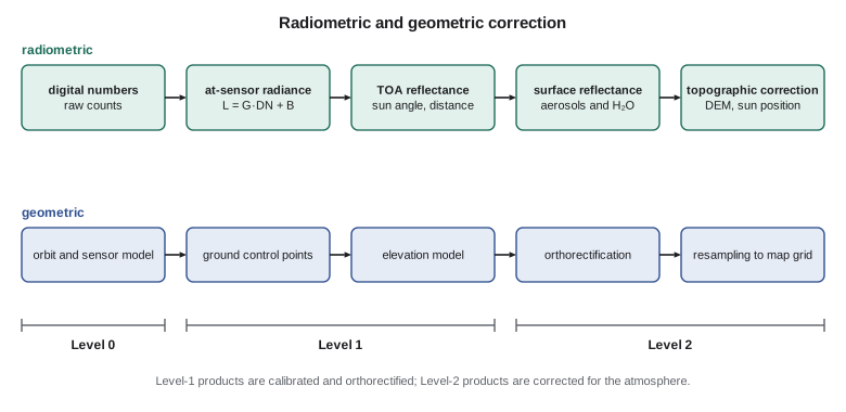
Satellite data are distributed at standard processing levels. Level 0 is raw instrument data. Level 1 products are calibrated and geolocated: Landsat Level-1 products are orthorectified using ground control and a digital elevation model and are delivered as scaled digital numbers with coefficients for conversion to top-of-atmosphere radiance and reflectance; Sentinel-2 Level-1C products are orthorectified top-of-atmosphere reflectance in 100 km tiles. Level 2 products are corrected for the atmosphere: Landsat Collection 2 Level-2 products provide surface reflectance and surface temperature, and Sentinel-2 Level-2A products provide surface reflectance with a scene classification layer marking cloud, shadow, snow and water. Level 3 and higher products are derived variables mapped on grids, such as composites, vegetation indices, land cover or evapotranspiration.

From digital numbers to radiance and reflectance

A detector produces a voltage proportional to the radiance falling on it, which is digitized to a digital number (DN). Calibration converts DN to at-sensor spectral radiance with a gain and an offset for each band, \(L = G \cdot DN + B\), determined before launch and maintained in orbit with onboard sources, solar diffusers, lunar views and vicarious calibration over stable sites. For pushbroom sensors each detector has its own coefficients, and errors in their relative calibration cause striping.

Radiance depends on the illumination, so for comparison between dates it is converted to top-of-atmosphere (TOA) reflectance, the reflectance the surface would have if there were no atmosphere:

Here \(d\) is the Earth-Sun distance in astronomical units, about 0.983 in early January and 1.017 in early July, \(E_{sun}\) is the mean exoatmospheric solar irradiance in the band, and \(\theta_s\) is the solar zenith angle. For Landsat products the metadata give reflectance rescaling coefficients directly, so that \(\rho_{TOA} = (M_\rho \cdot DN + A_\rho)/\sin\theta_{elev}\), where \(\theta_{elev}\) is the sun elevation; the division by the sine of the sun elevation corrects for the solar angle, while the Earth-Sun distance is already included in the coefficients. Theo's error had been to compare a TOA reflectance image from June with a surface reflectance image from July; the two are not comparable, especially through smoke.

Atmospheric correction

Atmospheric correction removes path radiance and the attenuation of the signal, using the radiative transfer relation of Lesson 1. Two broad approaches are used. Image-based methods use information within the image. The simplest is dark-object subtraction, which assumes that the darkest pixels in each band, such as deep shadow or clear deep water in the NIR, should have nearly zero reflectance, and that their recorded value is therefore path radiance to be subtracted from the whole band. It is fast and needs no outside data, but it ignores transmittance and assumes the haze is uniform. Model-based methods use radiative transfer codes with estimates of aerosol optical depth, water vapor, ozone and surface elevation, derived from the image itself, from the sensor's own atmospheric bands or from external data, and invert the full equation. The standard Level-2 products are produced this way, and their accuracy is typically a few thousandths to a few hundredths in reflectance, best over dark vegetated surfaces in clear air and poorest over bright surfaces, in heavy smoke and near cloud.

Because smoke is variable over short distances and its optical properties differ from the typical aerosol models, images taken through heavy smoke are often unreliable even after correction. The district's procedure, Leah decided, would record the aerosol optical depth reported with each Level-2 scene and exclude scenes above a threshold from quantitative products, while still using them for visual checks of flooding or fire.

Clouds, shadows and masks

Clouds and their shadows must be identified and removed before any quantitative analysis. Cloud detection uses the brightness of clouds in the visible, their low temperature in the thermal band, the cirrus band at 1.38 µm and their texture; shadows are found by projecting each cloud along the sun direction to the ground using an estimated cloud height. Standard products include cloud and shadow masks, such as the quality assessment bands of Landsat and the scene classification layer of Sentinel-2. These masks miss thin cloud, haze and shadow edges, and they can misclassify bright features, such as gravel pits and new concrete, as cloud. Most programs therefore dilate the mask by a few pixels and inspect suspicious changes before reporting them.

Topographic and directional effects

On slopes, the local angle between the sun and the surface normal changes the illumination. A coulee wall facing the sun is brighter than the same grass on a wall facing away, even though the vegetation is identical. Topographic correction uses a digital elevation model to compute the local illumination angle \(i\) and adjust the reflectance. The simple cosine correction, \(\rho_h = \rho \cos\theta_s / \cos i\), over-corrects faintly lit slopes, because it ignores diffuse skylight; methods such as the C-correction add an empirical constant estimated from the image. In the largely flat irrigated fields of the service area topographic effects are small, but on the coulee banks they dominate.

Directional effects arise because surfaces do not reflect equally in all directions. Across a wide swath, the view angle varies, and reflectance near the backscatter direction, where shadows are hidden, is higher than in the forward direction. For Landsat's narrow 185 km swath the effect is modest; for wide-swath sensors it can be large. Harmonized products that combine Landsat and Sentinel-2 normalize reflectance to a standard nadir view and a standard sun angle to reduce these differences, and also adjust for the small differences between the two sensors' bands.

import math
def T(A): return [list(r) for r in zip(*A)]
def mul(A, B): return [[sum(a * b for a, b in zip(r, c)) for c in zip(*B)] for r in A]
def inv(A):
    n = len(A); M = [list(map(float, r)) + [1.0 if i == j else 0.0 for j in range(n)] for i, r in enumerate(A)]
    for c in range(n):
        p = max(range(c, n), key=lambda r: abs(M[r][c])); M[c], M[p] = M[p], M[c]
        d = M[c][c]; M[c] = [x / d for x in M[c]]
        for r in range(n):
            if r != c:
                f = M[r][c]; M[r] = [x - f * y for x, y in zip(M[r], M[c])]
    return [r[n:] for r in M]
def diag(v): return [[v[i] if i == j else 0.0 for j in range(len(v))] for i in range(len(v))]
def col(v): return [[x] for x in v]
# 1. Digital number to top-of-atmosphere reflectance (NIR band) with Landsat-style rescaling factors
M_rho, A_rho = 2.0e-5, -0.1        # reflectance multiplicative and additive factors from the metadata
sun_elev = 61.3                    # degrees, from the metadata for the July scene
dn = {"canal water": 7620, "alfalfa": 30210, "stubble": 17840, "deep shadow in the coulee": 6150}
print("pixel                       DN      TOA reflectance")
toa = {}
for k, v in dn.items():
    rho = (M_rho * v + A_rho) / math.sin(math.radians(sun_elev))
    toa[k] = rho
    print(f"{k:26s} {v:6d}    {rho:7.4f}")

# 2. Dark-object subtraction: the darkest shadow should be nearly zero; treat its value as haze
haze = toa["deep shadow in the coulee"] - 0.01      # allow 1 % true reflectance in shadow
print(f"\nhaze estimate {haze:.4f}")
for k, v in toa.items():
    print(f"{k:26s} corrected {v - haze:7.4f}")

# 3. Radiance form: L = gain*DN + offset, then rho = pi L d^2 / (ESUN cos(theta_s))
gain, offset, esun, d = 0.010, -61.0, 1550.0, 1.0164   # W m-2 sr-1 um-1 per DN; Earth-Sun distance in AU (July)
L = gain * dn["alfalfa"] + offset
rho = math.pi * L * d**2 / (esun * math.cos(math.radians(90 - sun_elev)))
print(f"\nalfalfa radiance {L:.1f} W m-2 sr-1 um-1 -> reflectance {rho:.4f}")

# 4. Geometric correction: affine transformation from image (col, row) to project grid (E, N) by least squares
gcp = [  # col, row, E, N  (bridge corners, canal checks, road intersections)
    (112.4, 85.1, 385549.0, 5506785.9), (1840.7, 102.9, 437390.6, 5506936.5),
    (1795.2, 1610.3, 436654.5, 5461711.6), (140.8, 1588.6, 387045.7, 5461715.4),
    (980.3, 840.2, 411905.3, 5484491.5), (520.6, 1210.4, 398270.9, 5473206.6),
    (1402.1, 460.7, 424381.0, 5496045.3)]
Aa = [[1.0, c, r] for c, r, E, N in gcp]
At = T(Aa); N_ = inv(mul(At, Aa))
cE = mul(N_, mul(At, col([E for c, r, E, N in gcp])))
cN = mul(N_, mul(At, col([N for c, r, E, N in gcp])))
print("\nE = %.2f %+.4f col %+.4f row" % (cE[0][0], cE[1][0], cE[2][0]))
print("N = %.2f %+.4f col %+.4f row" % (cN[0][0], cN[1][0], cN[2][0]))
ss = 0.0
for c, r, E, N in gcp:
    vE = cE[0][0] + cE[1][0] * c + cE[2][0] * r - E
    vN = cN[0][0] + cN[1][0] * c + cN[2][0] * r - N
    ss += vE**2 + vN**2
    print(f"  GCP at col {c:7.1f} row {r:7.1f}: residual E {vE:6.2f} m  N {vN:6.2f} m")
rmse = math.sqrt(ss / len(gcp))
print(f"radial RMSE of the fit {rmse:.2f} m ({rmse / 30:.2f} pixel of 30 m)")

pixel                       DN      TOA reflectance
canal water                  7620     0.0597
alfalfa                     30210     0.5748
stubble                     17840     0.2928
deep shadow in the coulee    6150     0.0262

haze estimate 0.0162
canal water                corrected  0.0435
alfalfa                    corrected  0.5586
stubble                    corrected  0.2765
deep shadow in the coulee  corrected  0.0100

alfalfa radiance 241.1 W m-2 sr-1 um-1 -> reflectance 0.5755

E = 382147.69 +29.9855 col +0.4237 row
N = 5509298.60 +0.3948 col -29.9887 row
  GCP at col   112.4 row    85.1: residual E   5.11 m  N   5.05 m
  GCP at col  1840.7 row   102.9: residual E  -5.05 m  N   3.06 m
  GCP at col  1795.2 row  1610.3: residual E   5.33 m  N   5.05 m
  GCP at col   140.8 row  1588.6: residual E  -3.03 m  N  -1.23 m
  GCP at col   980.3 row   840.2: residual E  -6.89 m  N  -2.32 m
  GCP at col   520.6 row  1210.4: residual E   0.02 m  N  -0.74 m
  GCP at col  1402.1 row   460.7: residual E   4.51 m  N  -8.87 m
radial RMSE of the fit 6.58 m (0.22 pixel of 30 m)

The code shows the radiometric steps on four pixels. The deep shadow on the coulee wall, with a TOA reflectance of 0.026, is assumed to have a true reflectance of about 0.01, so 0.016 is attributed to haze and subtracted from every pixel in the band. The radiance form of the equation, with the July Earth-Sun distance of 1.016 AU, gives the same reflectance for the alfalfa as the rescaling coefficients, as it should. The geometric part is discussed below.

Geometric correction

Geometric correction places each pixel at its correct position on a map projection. Two approaches are used. Empirical correction fits a transformation between image coordinates (column and row) and map coordinates using ground control points (GCPs): well-defined features visible in the image whose coordinates are known, such as road intersections, bridge corners and canal structures. The transformation may be affine, with six parameters for translation, rotation, scale and shear, or a polynomial of second or third order for more complex distortion. It is fitted by least squares, and the residuals at the GCPs and, more importantly, the errors at independent checkpoints describe its accuracy. Polynomials fit well at the GCPs and can behave badly between and beyond them, so a higher order is justified only with many well-distributed points.

Rigorous correction, or orthorectification, uses a model of the sensor's geometry, the satellite's orbit and attitude and a digital elevation model to compute where each ground point appears in the image, correcting relief displacement as well as the systematic distortions. Landsat and Sentinel-2 products are orthorectified by the providers with a geolocation accuracy of roughly 10 to 15 m or better, and Sentinel-2 tiles are now aligned to a global reference image so that images from different dates overlay within a fraction of a pixel. High-resolution commercial images are delivered with rational polynomial coefficients, a generic replacement for the rigorous sensor model, and are orthorectified by the user with a few GCPs and a DEM.

The overlay problem Theo found was traced to a parcel map in a different datum: the district's legacy parcel lines were in NAD27, while the Landsat products were in WGS 84, which in this region agrees with NAD83(2011) to about a meter or two. The difference between NAD27 and NAD83 near Great Falls is tens of meters, almost two Landsat pixels. Once the parcels were transformed to NAD83(2011) in the project grid, the boundaries fell into place. The lesson from the geodesy course applied directly: before blaming the image, check the datum and projection of everything being overlaid.

Resampling

After the transformation is known, the output image is built on a regular map grid by computing for each output pixel where it falls in the input image and interpolating a value there. Nearest-neighbor resampling takes the value of the closest input pixel; it preserves the original values, which matters for classified images and quality flags, but produces a blocky appearance and can shift features by up to half a pixel. Bilinear interpolation uses the four nearest pixels and gives a smoother image but blends values. Cubic convolution uses sixteen pixels and gives the sharpest appearance at the cost of some overshoot at edges. Radiometric analysis is best done on the original pixel grid or with as few resampling steps as possible, because each resampling smooths and slightly alters the data.