
GEOM-200 · Lesson 9 of 12 · 21 min
Geographic information systems
A geographic information system (GIS) stores, analyses and displays information tied to locations. It is where the products of surveying, photogrammetry, lidar and remote sensing come together with information from many other sources: property boundaries, zoning, utilities, soils, census data, traffic counts, environmental sensitivities and asset condition. Municipalities run their water and sewer networks from GIS; irrigation districts track canals and turnouts in it; pipeline companies plan routes and manage integrity with it; and emergency services dispatch from it. This lesson introduces how GIS represents the world, the two main data models, attributes and topology, coordinate systems in GIS, metadata and quality, and the core analysis operations of selection, buffering and overlay, with a pure-Python example that shows what the software is doing underneath. CIV-250 lesson 11 places GIS within a surveying project; GEOM-330 Geographic Information Systems develops spatial analysis and databases in depth.
What makes data geographic
Geographic data combine three things: where a feature is (its geometry), what it is (its attributes) and when the information was true (its time). A water main, for example, has a line geometry, attributes such as material, diameter, installation year and condition rating, and a date of the last inspection. The power of GIS comes from linking these: finding all cast-iron mains more than 60 years old within 50 m of a school, say, takes seconds in a GIS and days with paper maps.
Every GIS layer must be in a known coordinate reference system, as described in lesson 3, with its datum, projection, units and, for high-accuracy work, epoch stated. Most GIS software can reproject data on the fly for display, but analysis such as measuring areas or buffering should be done in a projected system with suitable distortion characteristics, not in latitude and longitude degrees, where a degree of longitude is not the same distance as a degree of latitude.
Vector and raster
GIS uses two main ways of representing the world. The vector model represents discrete features as points, lines and polygons defined by coordinates. A survey monument is a point; a road centerline is a line; a parcel is a polygon. The raster model divides space into a regular grid of cells, each holding a value. A digital terrain model, an orthophoto and a land cover classification are all rasters.
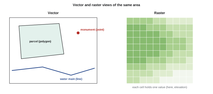
| Vector | Raster | |
|---|---|---|
| Represents | Discrete features with exact boundaries | Continuous surfaces and imagery |
| Precision | As precise as the coordinates | Limited by cell size |
| Typical data | Parcels, roads, utilities, survey points | Elevation, imagery, land cover, rainfall |
| Analysis strengths | Networks, topology, precise overlay | Surface analysis, map algebra, modeling |
| Storage | Compact for sparse features | Large for fine cells over big areas |
Most projects use both. A floodplain study combines a lidar raster terrain model with vector river centerlines, cross-section lines and parcel polygons. Raster cell size must suit the analysis: a 1 m terrain model is good for grading, a 30 m land cover map is good for watershed studies but useless for individual lots.
Point clouds from lidar and photogrammetry are a third kind of data, neither grid nor simple vector, and modern GIS and specialized software handle them directly. Three-dimensional city models, building information models and digital twins of infrastructure extend GIS into the third dimension and connect it with design software.
Attributes, tables and databases
Each vector feature has a row in an attribute table, with columns for its properties. Tables can be joined to other tables using a common key, such as a parcel identifier or an asset number, so that information maintained by different departments can be brought together. Professional GIS stores data in spatial databases, which handle many users editing at once, keep histories of changes and enforce rules about valid values. Open standards, including those of the Open Geospatial Consortium, define common formats and web services so that data can move between systems: GeoPackage for files, web map and feature services for sharing data online, and well-known text for describing geometries and coordinate systems.
Topology
Topology describes how features relate to one another: which parcels share a boundary, which pipes connect at a valve, which roads meet at an intersection. A GIS that maintains topology can enforce rules such as parcels must not overlap, parcels must not leave gaps, and every pipe must connect to another pipe or a structure. Topology errors are among the commonest problems in data converted from drawings, where lines that look joined actually miss by a few millimeters, or overlap. Network topology allows tracing analyses: which customers lose water if this valve is closed, or which way does stormwater flow from this inlet.
Spatial analysis
Analysis is what distinguishes a GIS from a digital map. The basic operations are few but combine into powerful workflows.
| Operation | What it does | Example |
|---|---|---|
| Attribute query | Selects features by their properties | All mains installed before 1960 |
| Spatial query | Selects features by location | All parcels within the floodplain |
| Buffer | Creates zones at a set distance from features | 30 m setback from a watercourse |
| Overlay | Combines layers geometrically | Area of each parcel inside the setback |
| Network analysis | Routes and traces along connected lines | Shortest route for a utility crew |
| Surface analysis | Derives slope, aspect, watersheds and volumes from rasters | Drainage areas for a stormwater design |
| Interpolation | Estimates values between sample points | Groundwater surface from well levels |
A buffer around a point is a circle; around a line, a corridor with rounded ends; around a polygon, the polygon enlarged outward. Overlay operations include intersection, which keeps only the area common to both layers, union, which keeps everything and splits it where boundaries cross, and difference, which removes one layer from another. Each output feature carries the attributes of the inputs, so an intersection of parcels with a setback buffer gives, for each parcel, the area affected.
Worked problem
Setback areas on Coulee Ridge
The municipality requires a 30 m environmental setback from the top of the coulee bank along the east side of the Coulee Ridge subdivision. Marcus has the top-of-bank line from the survey and the lot polygons from the subdivision design. Lot 14 is a rectangle 25 m wide (east–west) and 40 m deep (north–south), and its east side lies 12 m from the top of bank, which runs straight north–south. How much of Lot 14 lies inside the setback?
Show solution
- \[\text{setback reaches } 30 - 12 = 18\ \text{m into the lot from its east side}\]
- \[\text{affected area} = 18 \times 40 = 720\ \text{m}^2\]
- \[\text{lot area} = 25 \times 40 = 1\,000\ \text{m}^2\]
- \[\text{share} = \frac{720}{1000} = 72\ \text{percent}\]
Answer: Almost three-quarters of the lot falls in the setback, which leaves too little room for a house. The design team uses the GIS overlay to test several lot layouts along the bank before the subdivision plan is finalized.
Buffer and overlay in pure Python
GIS packages hide the geometry behind menus, but the underlying operations are straightforward computational geometry. The script below uses no GIS library. It approximates a buffer around a line as a polygon, clips a lot polygon to the buffer using the Sutherland–Hodgman algorithm, computes areas with the shoelace formula, and runs a point-in-polygon test to find which survey points lie in the setback.
# Buffer, clip (intersection), area and point-in-polygon in plain Python
import math

def area(poly):
    s = 0.0
    for (x1, y1), (x2, y2) in zip(poly, poly[1:] + poly[:1]):
        s += x1 * y2 - x2 * y1
    return abs(s) / 2

def buffer_segment(p, q, d, n=16):
    # Polygon around segment p-q at distance d, with rounded ends (counter-clockwise)
    ang = math.atan2(q[1] - p[1], q[0] - p[0])
    pts = []
    for k in range(n + 1):                      # half circle around q
        a = ang - math.pi / 2 + math.pi * k / n
        pts.append((q[0] + d * math.cos(a), q[1] + d * math.sin(a)))
    for k in range(n + 1):                      # half circle around p
        a = ang + math.pi / 2 + math.pi * k / n
        pts.append((p[0] + d * math.cos(a), p[1] + d * math.sin(a)))
    return pts

def clip(subject, clipper):
    # Sutherland-Hodgman: clip any polygon by a convex counter-clockwise polygon
    def inside(pt, a, b):
        return (b[0] - a[0]) * (pt[1] - a[1]) - (b[1] - a[1]) * (pt[0] - a[0]) >= 0
    def cross_point(s, e, a, b):
        dc = (a[0] - b[0], a[1] - b[1]); dp = (s[0] - e[0], s[1] - e[1])
        n1 = a[0] * b[1] - a[1] * b[0]; n2 = s[0] * e[1] - s[1] * e[0]
        den = dc[0] * dp[1] - dc[1] * dp[0]
        return ((n1 * dp[0] - n2 * dc[0]) / den, (n1 * dp[1] - n2 * dc[1]) / den)
    out = subject
    for a, b in zip(clipper, clipper[1:] + clipper[:1]):
        inp, out = out, []
        if not inp:
            break
        s = inp[-1]
        for e in inp:
            if inside(e, a, b):
                if not inside(s, a, b):
                    out.append(cross_point(s, e, a, b))
                out.append(e)
            elif inside(s, a, b):
                out.append(cross_point(s, e, a, b))
            s = e
    return out

def point_in_polygon(pt, poly):
    x, y, inside = pt[0], pt[1], False
    for (x1, y1), (x2, y2) in zip(poly, poly[1:] + poly[:1]):
        if (y1 > y) != (y2 > y) and x < x1 + (y - y1) * (x2 - x1) / (y2 - y1):
            inside = not inside
    return inside

# Top of bank runs north-south at x = 137; Lot 14 spans x 100-125, y 0-40 (local coordinates in m)
bank = ((137.0, -60.0), (137.0, 100.0))
setback = buffer_segment(bank[0], bank[1], 30.0, n=32)
lot14 = [(100.0, 0.0), (125.0, 0.0), (125.0, 40.0), (100.0, 40.0)]
inter = clip(lot14, setback)
print(f"Lot 14 area {area(lot14):.1f} m2, inside setback {area(inter):.1f} m2 "
      f"({100 * area(inter) / area(lot14):.0f}%)")

# A bend in the bank: buffer each segment and test survey points against the union
bank2 = [(137.0, -60.0), (137.0, 20.0), (120.0, 70.0)]
zones = [buffer_segment(a, b, 30.0, n=32) for a, b in zip(bank2, bank2[1:])]
points = {"BH-1 borehole": (101.0, 5.0), "BH-2 borehole": (112.0, 30.0),
          "Lot 15 corner": (100.0, 80.0), "Pond outlet": (90.0, 95.0)}
for name, p in points.items():
    hit = any(point_in_polygon(p, z) for z in zones)
print(f"{name:14s} {'inside' if hit else 'outside'} the setback")Lot 14 area 1000.0 m2, inside setback 720.0 m2 (72%) BH-1 borehole outside the setback BH-2 borehole inside the setback Lot 15 corner inside the setback Pond outlet outside the setback
The clipped area matches the hand calculation of 720 m², a useful check that the code is right. For the bent bank line, each segment is buffered separately and a point is in the setback if it falls in any of the pieces, which is how a union behaves for this test. A full GIS adds robust handling of awkward cases, such as polygons with holes, curved boundaries and points exactly on an edge, but the principles are the same, and knowing them helps a geomatics engineer understand why tiny gaps, slivers and overlaps appear when layers from different sources are overlaid.
Data quality and metadata
GIS makes it easy to combine data of very different quality, and the result is only as good as the weakest layer. A parcel layer digitized from old paper maps may be several meters out compared with a modern survey, so overlaying it on a centimeter-accurate lidar model can produce misleading results: houses appear to sit in the street and boundaries cut through buildings. Data quality has several components: positional accuracy, attribute accuracy, completeness, logical consistency (such as valid topology), currency and lineage, the record of where the data came from and what was done to it.
Metadata, data about the data, records these properties, along with the coordinate system, the date, the custodian and any limitations on use. Standards such as ISO 19115 define what metadata should contain. Good metadata lets a future user decide whether a layer is fit for their purpose; missing metadata is one of the commonest reasons good data cannot be reused.
In the US, deeds, recorded plats and surveys are the authoritative sources for property boundaries; the parcel layer in a county or state GIS is a representation for taxation, planning and mapping, not a legal survey. Montana maintains a statewide cadastral parcel layer built from county records, and cities such as Great Falls build their own GIS layers on it. The legal boundary is what the survey and recorded documents establish, as lesson 11 explains.
GIS in engineering practice
For a geomatics engineer, GIS is both a client and a product. Survey data feed GIS: control points, as-built utilities, topographic features and boundaries. GIS in turn supports surveying and engineering: searching for records before a survey, planning flights and field work, analyzing alternatives for a route and presenting results to the public. At Coulee Geomatics, Marcus maintains the GIS for the irrigation district under a service contract, updating canal and structure records from field surveys each fall and producing condition maps that set the following year's maintenance program.
Web GIS has made spatial information widely available: interactive maps on municipal websites, field apps that let crews view and edit data on tablets, and dashboards that show the status of work in real time. With wider access comes responsibility for privacy and security. Detailed locations of critical infrastructure, personal information attached to addresses and the locations of sensitive species are restricted, and GIS professionals decide what to publish and at what level of detail.
Common mistakes
MistakeMeasuring areas and buffers in latitude and longitude degrees.
InsteadProject the data to a suitable projected coordinate system first.
MistakeOverlaying layers of very different accuracy without noting it.
InsteadCheck and record the accuracy and lineage of each layer.
MistakeTreating GIS parcels as legal boundaries.
InsteadUse the survey and registered or recorded documents for legal boundaries.
MistakeIgnoring topology errors from converted drawings.
InsteadRun topology checks for gaps, overlaps and unconnected lines.
Summary and key terms
- GIS links geometry, attributes and time for features and surfaces.
- Vector data model discrete features; raster data model continuous surfaces and imagery.
- Topology records how features connect and enforces rules about gaps and overlaps.
- Buffer, overlay, query, network and surface analysis are the core operations.
- Data quality includes accuracy, completeness, consistency, currency and lineage.
- GIS parcel layers represent boundaries but do not define them legally.
- GIS
- A geographic information system for storing, analyzing and displaying located information.
- Vector
- A data model using points, lines and polygons defined by coordinates.
- Raster
- A data model using a regular grid of cells with values.
- Topology
- The rules and records of how features connect and share boundaries.
- Buffer
- A zone at a set distance around a feature.
- Overlay
- Combining layers geometrically, as by intersection or union.
- Metadata
- Information describing a dataset’s content, quality, coordinate system and origin.
Practice problems
Work each problem on paper first, then reveal the answer to check.
A lot 30 m by 45 m has its long side 10 m from a creek, with a 25 m setback. What area is in the setback?
Show answer
\(15 \times 45 = 675\) m².
Why should buffers be computed in a projected system?
Show answer
Distances in degrees vary with direction and latitude, so buffers would be distorted.
Give one example each of vector and raster data.
Show answer
Vector: parcels or pipes; raster: elevation or imagery.
What does a network trace answer in a water GIS?
Show answer
Which pipes and customers are affected when a valve is closed, or which way flow travels.
Name three components of data quality.
Show answer
Positional accuracy, completeness and lineage, among others.
Lesson quiz · 5 questions
Score 60% or more to complete this lesson.
Create a free account to save your progress, take quizzes and earn a certificate.