
GEOM-200 · Lesson 7 of 12 · 22 min
Photogrammetry and remote sensing
Most of the maps used today were not drawn by walking the ground but measured from images. Photogrammetry is the science of making reliable measurements from photographs, and remote sensing is the wider field of gathering information about the Earth's surface from sensors that are not in contact with it, on aircraft, drones and satellites. Together they produce orthophotos, topographic maps, elevation models, land cover maps, crop health indices, flood extents and change detection over decades. This lesson introduces the geometry of an image, the scale and ground sample distance that control what can be measured, how overlapping images become three-dimensional models, the electromagnetic spectrum and the main kinds of satellite and airborne sensor, and how geomatics engineers control and check the results. GEOM-310 Photogrammetry and GEOM-320 Remote Sensing take each half of the subject much further.
From pictures to measurements
Photogrammetry began almost as soon as photography itself. In the nineteenth century, surveyors measured from photographs taken from hilltops, and in Canada, Édouard Deville, the Surveyor General, used photographs taken from mountain peaks to map the Rocky Mountains in the 1880s and 1890s, one of the first large-scale uses of photogrammetry anywhere. Aerial photography from aircraft took over in the twentieth century, first with film cameras and optical-mechanical plotting instruments, then with analytical plotters that used computers, and since the 1990s with fully digital workflows. Today a drone carrying a consumer-sized camera can produce a centimeter-resolution orthophoto of a construction site in an afternoon, and computer vision algorithms do much of the matching that operators once did by eye.
The geometry of a vertical photograph
An aerial camera is close to a pinhole: light from each ground point passes through the center of the lens, the perspective center, and strikes the image sensor. For a truly vertical photograph over flat ground, similar triangles give the photo scale as the ratio of the focal length to the flying height above the ground.
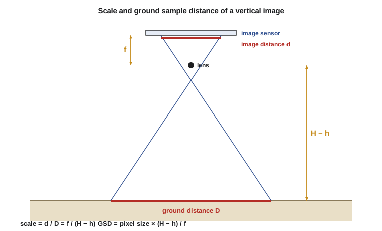
where \(f\) is the focal length, \(H\) the flying height above the datum, \(h\) the ground elevation and \(p\) the size of one pixel on the sensor. The ground sample distance (GSD) is the size of one pixel on the ground, and it is the most important number in any imaging project, because it controls what can be seen and how accurately points can be measured. As a rule of thumb, well-controlled photogrammetry can measure horizontal positions to about one to two times the GSD and heights to about two to three times the GSD.
Real ground is not flat, and real photographs are never exactly vertical. Points higher than the average ground appear displaced outward from the center of the photograph, an effect called relief displacement. That is why a raw aerial photograph is not a map: tall buildings lean outward, and hills are stretched. The displacement grows with the height of the object and its distance from the photo center:
where \(d\) is the displacement on the image, \(r\) the radial distance of the top of the object from the image center and \(h_o\) the height of the object. Relief displacement is a nuisance for map making but a gift for measurement, because it lets heights be measured from images.
Worked problem
Planning a drone flight for the Coulee Ridge subdivision
Ines plans a drone survey of the 64 ha Coulee Ridge subdivision site to produce an orthophoto and a surface model. The camera has a focal length of 8.8 mm, a sensor 13.2 mm × 8.8 mm with 5,472 × 3,648 pixels, and the site needs a GSD of 2.5 cm. Find the flying height above ground, the ground footprint of each image and the spacing between exposures for 75 percent forward overlap.
Show solution
- \[p = \frac{13.2\ \text{mm}}{5472} = 0.002412\ \text{mm} = 2.412\ \mu\text{m}\]
- \[H - h = \frac{\text{GSD} \times f}{p} = \frac{0.025 \times 8.8}{0.002412} = 91.2\ \text{m}\]
- \[\text{footprint} = 5472 \times 0.025 = 136.8\ \text{m across}, \quad 3648 \times 0.025 = 91.2\ \text{m along track}\]
- \[\text{exposure spacing} = (1 - 0.75) \times 91.2 = 22.8\ \text{m}\]
Answer: The drone flies at about 91 m above ground, below the usual 122 m (400 ft) limit for small drones in both Canada and the US, and takes an image every 22.8 m along each line. With 65 percent side overlap, the flight lines are \((1 - 0.65) \times 136.8 = 47.9\) m apart.
Stereo and three dimensions
A single photograph records directions from the camera to ground points but not distances. Two photographs taken from different positions, with the same ground in view, allow each point to be found where the two rays intersect, just as human eyes judge depth. Aerial surveys are therefore flown in strips with a forward overlap between consecutive photographs, traditionally 60 percent and now often 75 to 80 percent for drones, and a side overlap between strips of 30 to 70 percent.
The difference in a point's position between the two images is called parallax, and it depends on the point's height: higher points have larger parallax. For a pair of vertical images, the height of a point is found from the measured parallax, the distance between the two camera positions (the air base) and the focal length.
To turn many overlapping images into a model, photogrammetry must know the position and orientation of the camera at each exposure (exterior orientation) and the internal geometry of the camera: focal length, the position of the principal point and lens distortion (interior orientation). Bundle adjustment solves for all of these together, by least squares, using thousands of tie points that appear in several images and a few ground control points whose coordinates are known. Modern software finds tie points automatically by matching image features, in a process often called structure from motion, and then matches nearly every pixel to produce a dense point cloud.
Products of photogrammetry
| Product | What it is | Typical uses |
|---|---|---|
| Orthophoto (orthomosaic) | Images corrected for relief and tilt so that scale is uniform | Base maps, site plans, GIS backdrop |
| Digital surface model (DSM) | Heights of the top surface, including buildings and trees | Volumes, line of sight, urban models |
| Digital terrain model (DTM) | Heights of the bare ground | Grading design, drainage, contours |
| Vector mapping | Features such as roads, buildings and fences digitized in 3D | Topographic maps, asset inventories |
| Point cloud | Millions of 3D points with color | Modeling, change detection |
An orthophoto is made by draping the images over a surface model and re-projecting each pixel straight down, removing relief displacement. If the surface model is a bare-ground DTM, buildings still lean in the result; a true orthophoto uses a DSM so that roofs sit exactly over footprints. Ground control and independent check points are essential. Control points fix the model to the ground; check points, which are not used in the adjustment, show how accurate the result really is. Coulee Geomatics sets at least five control targets and a similar number of check targets on every drone job, measured by RTK GNSS from site control.
The electromagnetic spectrum
Remote sensing extends photogrammetry beyond visible light. Every material reflects, absorbs and emits electromagnetic energy differently at different wavelengths, its spectral signature. Healthy vegetation, for example, absorbs red light strongly for photosynthesis and reflects near-infrared light strongly from leaf cell structure, while water absorbs near-infrared almost completely. Sensors that record several wavelength bands can therefore tell crops from bare soil, water from land and stressed vegetation from healthy plants.
| Region | Wavelengths | What it shows |
|---|---|---|
| Visible | 0.4–0.7 µm | What the eye sees: color, texture |
| Near-infrared | 0.7–1.3 µm | Vegetation health and biomass, water boundaries |
| Shortwave infrared | 1.3–3 µm | Moisture in soil and plants, minerals, burn scars |
| Thermal infrared | 8–14 µm | Surface temperature, heat loss, water discharges |
| Microwave (radar) | 1 mm–1 m | Surface roughness and moisture, through cloud and at night |
A widely used measure of vegetation is the normalized difference vegetation index, computed from the near-infrared and red reflectances. It ranges from about −1 to 1, with dense healthy vegetation above about 0.6, bare soil near 0.1 to 0.2 and water below zero.
Satellites and sensors
Remote sensing sensors are either passive, recording reflected sunlight or emitted heat, or active, sending out their own energy and recording what returns. Optical cameras and multispectral scanners are passive; radar and lidar are active. Passive optical sensors need daylight and clear skies. Synthetic aperture radar (SAR) works day and night through cloud, and interferometric SAR (InSAR) compares radar phase between passes to measure ground movement of millimeters over large areas, which is used to monitor subsidence, landslides, mines and infrastructure.
Satellite imagery is described by four kinds of resolution. Spatial resolution is the GSD, from about 30 cm for the best commercial satellites to 10 to 30 m for free government missions and a kilometer for weather satellites. Spectral resolution is the number and width of the bands, from a few broad bands to hundreds of narrow ones in hyperspectral sensors. Temporal resolution is how often the same place is imaged, from several times a day to every couple of weeks. Radiometric resolution is how finely brightness is recorded.
The Landsat program, operated by NASA and the US Geological Survey, has imaged the Earth since 1972 and provides the longest continuous record of land change, free of charge. The European Space Agency's Sentinel-2 satellites provide 10 m multispectral imagery every few days, also free. The US Department of Agriculture's National Agriculture Imagery Program flies leaf-on aerial imagery of the country, the USGS runs the 3D Elevation Program, and NOAA's weather and ocean satellites support forecasting and coastal mapping. In Montana, satellite imagery is used to monitor drought, wildfire burn scars, irrigation and rangeland condition.
Image processing and classification
Raw satellite images need geometric correction, to place each pixel on the map, and often radiometric and atmospheric correction, so that values represent surface reflectance rather than whatever reached the sensor through haze. Classification then turns pixel values into categories. In supervised classification, an analyst provides training areas of known land cover and an algorithm assigns every other pixel to the most similar class. Unsupervised classification groups pixels by similarity and lets the analyst name the groups. Machine learning methods, including deep neural networks, now dominate both pixel and object classification, and can find buildings, roads and trees in imagery automatically.
Every classified map needs an accuracy assessment, comparing a sample of mapped pixels with reference data from field visits or higher-resolution imagery. The result is a confusion matrix, from which overall accuracy and the accuracy of each class are computed. A land cover map that claims 90 percent overall accuracy may still be poor for a rare class such as wetlands, which is often the class that matters most for an environmental assessment.
# Photo scale, ground sample distance and flight plan, then NDVI for sample pixels
f_mm, sensor_w_mm, px_w, px_h = 8.8, 13.2, 5472, 3648
pixel_mm = sensor_w_mm / px_w

for gsd_cm in (1.5, 2.5, 5.0):
    agl = (gsd_cm / 100) * f_mm / pixel_mm
    across, along = px_w * gsd_cm / 100, px_h * gsd_cm / 100
    spacing = (1 - 0.75) * along
    line_gap = (1 - 0.65) * across
    scale = agl / (f_mm / 1000)
    print(f"GSD {gsd_cm:.1f} cm: fly {agl:6.1f} m AGL, scale 1:{scale:,.0f}, "
          f"footprint {across:.0f} x {along:.0f} m, shots every {spacing:.1f} m, lines {line_gap:.1f} m apart")

# Images needed for a 800 m x 800 m (64 ha) site at 2.5 cm
import math
gsd = 0.025
across, along = px_w * gsd, px_h * gsd
lines = math.ceil(800 / ((1 - 0.65) * across)) + 1
shots = math.ceil(800 / ((1 - 0.75) * along)) + 1
print(f"64 ha site at 2.5 cm: {lines} lines x {shots} shots = {lines * shots} images")

# Relief displacement of a 12 m grain elevator 40 mm from the principal point at 1:10,000
H_agl, f = 880.0, 0.088
r_mm, h_obj = 40.0, 12.0
d_mm = r_mm * h_obj / H_agl
print(f"Relief displacement: {d_mm:.2f} mm on the image = {d_mm / 1000 * H_agl / f:.2f} m on the ground")

# NDVI from red and near-infrared reflectance
samples = {"irrigated alfalfa": (0.05, 0.48), "dry stubble": (0.18, 0.26),
           "bare soil": (0.22, 0.28), "canal water": (0.06, 0.03)}
for name, (red, nir) in samples.items():
print(f"{name:18s} NDVI {(nir - red) / (nir + red):+.2f}")GSD 1.5 cm: fly 54.7 m AGL, scale 1:6,218, footprint 82 x 55 m, shots every 13.7 m, lines 28.7 m apart GSD 2.5 cm: fly 91.2 m AGL, scale 1:10,364, footprint 137 x 91 m, shots every 22.8 m, lines 47.9 m apart GSD 5.0 cm: fly 182.4 m AGL, scale 1:20,727, footprint 274 x 182 m, shots every 45.6 m, lines 95.8 m apart 64 ha site at 2.5 cm: 18 lines x 37 shots = 666 images Relief displacement: 0.55 mm on the image = 5.45 m on the ground irrigated alfalfa NDVI +0.81 dry stubble NDVI +0.18 bare soil NDVI +0.12 canal water NDVI -0.33
Halving the GSD halves the flying height, so it roughly quadruples the number of images and the processing time, which is why the GSD should be set by what the project really needs. The relief displacement line shows that a 12 m grain elevator near the edge of a 1:10,000 photograph appears shifted by about 0.55 mm on the image, which is about 5.5 m on the ground, enough to put its top over the neighboring lot on a large-scale map. The NDVI values separate irrigated alfalfa clearly from stubble, soil and canal water, the basis of irrigation monitoring for the irrigation district clients.
Accuracy standards
Geomatics firms in the US commonly specify and report photogrammetric and lidar accuracy using the ASPRS Positional Accuracy Standards for Digital Geospatial Data, which express accuracy as the root mean square error of independent check points against higher-accuracy survey values. Federal contracts, including those for the 3D Elevation Program, add their own requirements for control, check points and reporting.
The key principle in every standard is independence: the check points must be surveyed by a more accurate method and must not be used to fit the model. A report that quotes only the fit to the control points says how well the software adjusted, not how accurate the map is.
Common mistakes
MistakeChoosing a GSD finer than the project needs.
InsteadSet the GSD from the smallest feature and accuracy required.
MistakeTreating a raw photograph as a map.
InsteadUse orthophotos, which remove relief displacement and tilt.
MistakeUsing the same points for control and accuracy checks.
InsteadReserve independent check points measured by a more accurate method.
MistakeReading NDVI or classification maps without an accuracy assessment.
InsteadValidate with field or reference data, class by class.
Summary and key terms
- Photo scale is \(f/(H - h)\), and the ground sample distance is pixel size times flying height over focal length.
- Relief displacement moves high points outward from the image center and allows heights to be measured.
- Overlapping images, bundle adjustment and ground control produce 3D models and orthophotos.
- Different materials have different spectral signatures; NDVI uses red and near-infrared.
- Passive sensors record reflected or emitted energy; radar and lidar are active.
- Accuracy is proven with independent check points, not with the control fit.
- Photogrammetry
- The science of making measurements from images.
- Ground sample distance
- The size of one image pixel on the ground.
- Relief displacement
- The outward shift of an elevated point from the image center.
- Bundle adjustment
- A least squares solution for camera positions, orientations and ground points from many images.
- Orthophoto
- An image corrected for relief and tilt so that it has uniform scale.
- Spectral signature
- The pattern of reflectance of a material across wavelengths.
- Synthetic aperture radar
- An active microwave imaging system that works day and night through cloud.
Practice problems
Work each problem on paper first, then reveal the answer to check.
A camera with a 50 mm focal length flies 1,500 m above ground. What is the photo scale?
Show answer
\(0.05/1500 = 1{:}30\,000\).
Pixels are 4 µm and the focal length is 100 mm. What flying height above ground gives a 10 cm GSD?
Show answer
\(0.10 \times 0.1/0.000004 = 2\,500\) m.
A pixel has red reflectance 0.08 and NIR 0.40. Compute NDVI.
Show answer
\((0.40 - 0.08)/(0.40 + 0.08) = 0.67\).
Why are radar satellites useful for flood mapping?
Show answer
They see through cloud and at night, and smooth water reflects radar away, so it appears dark.
What is the difference between a DSM and a DTM?
Show answer
A DSM includes buildings and vegetation; a DTM is the bare ground.
Lesson quiz · 5 questions
Score 60% or more to complete this lesson.
Create a free account to save your progress, take quizzes and earn a certificate.