
GEOM-200 · Lesson 6 of 12 · 21 min
Satellite positioning
Global navigation satellite systems have changed geomatics more than any other technology since the electronic distance meter. A receiver the size of a paperback book can now give a position to a centimeter in seconds, anywhere with a view of the sky, in a global reference frame. The same signals guide farm tractors, construction machines and phones, synchronize power grids and financial networks, and monitor the slow movement of continents. This lesson explains how satellite positioning works, what limits its accuracy, the main positioning methods from a single phone to precise post-processing, and how geomatics engineers build reliable results from it. CIV-250 lesson 10 covers field procedures for static and RTK surveys; this lesson is about the system and the error budget behind those procedures, and GEOM-300 Satellite Positioning treats the observation equations and processing in full.
The constellations
Four global systems are in operation. GPS, run by the United States, was the first, with full operation in 1995. GLONASS is Russia's system. Galileo is the European Union's system, and BeiDou is China's. Regional systems add satellites over particular areas: Japan's QZSS and India's NavIC. Each global system has roughly 24 to 35 satellites in medium Earth orbit at altitudes of about 19,000 to 23,000 km, arranged so that at least four, and usually many more, are above the horizon everywhere at all times. A modern multi-constellation receiver in an open area typically tracks 25 to 40 satellites at once.
Each satellite carries atomic clocks and broadcasts signals on several frequencies in the L band, between about 1.1 and 1.6 GHz. The signals carry a ranging code, a pseudo-random sequence that lets the receiver measure the signal's travel time, and a navigation message that tells the receiver where the satellite is (its broadcast ephemeris) and how its clock is behaving. Control segments of ground stations track the satellites, compute their orbits and clocks and upload the navigation messages.
Measuring range by time
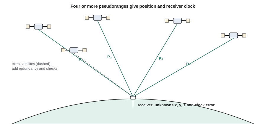
The receiver measures how long the signal took to arrive by comparing the received code with a copy generated inside the receiver. Multiplying that time by the speed of light gives a range. Because the receiver's clock is a cheap quartz oscillator, not an atomic clock, the measured range includes an unknown clock error that is the same for all satellites at a given moment. The measured value is therefore called a pseudorange.
where \(\rho\) is the true geometric range, \(c\) the speed of light, \(dt_r\) and \(dt^s\) the receiver and satellite clock errors, \(I\) and \(T\) the ionospheric and tropospheric delays and \(\varepsilon\) everything else, including multipath and noise. With four unknowns, three position coordinates and the receiver clock, at least four satellites are needed. With more, the receiver solves by least squares and can detect bad measurements.
A one-microsecond clock error is worth 300 m of range, which shows why solving for the clock is essential and why satellite clock errors must be known to within a few nanoseconds for meter-level positioning.
The error budget
A stand-alone receiver using code pseudoranges and broadcast orbits typically gets a horizontal position within a few meters. The error comes from several sources, which can be listed as a budget of user equivalent range errors:
| Source | Typical size (single frequency) | How it is reduced |
|---|---|---|
| Satellite orbit | 0.5–1 m | Precise orbits, differential corrections |
| Satellite clock | 0.5–1 m | Precise clocks, differencing |
| Ionosphere | 2–10 m (more in storms) | Dual frequency, models, differencing |
| Troposphere | 0.2–0.5 m after modeling | Models, estimation, differencing |
| Multipath | 0.2–2 m (code) | Site choice, antenna design, averaging |
| Receiver noise | 0.1–0.5 m (code) | Better receivers, carrier phase |
The ionosphere, the layer of charged particles 50 to 1,000 km up, delays the code and advances the carrier by an amount proportional to the inverse square of frequency. Measuring on two frequencies lets the receiver remove almost all of it. The troposphere, the lower atmosphere, delays signals by about 2.3 m at the zenith, and more at low elevations. Most of that is the predictable dry part; the smaller wet part depends on water vapor and must be modeled or estimated. Multipath, signals reflected from nearby surfaces, is the error most under the surveyor's control, through good site selection.
The range errors turn into position errors through the satellite geometry. When the visible satellites are spread across the sky, small range errors produce small position errors; when they are bunched together, the same range errors produce large position errors. The dilution of precision (DOP) numbers express this. The position error is approximately the DOP multiplied by the user equivalent range error.
Horizontal DOP (HDOP) is usually smaller than vertical DOP (VDOP), because satellites are only ever above the receiver, never below it. That is why GNSS heights are usually about one and a half to two times less precise than horizontal positions.
# GNSS position error budget: combine range errors and multiply by DOP
import math

budgets = {
    "Single-frequency code, broadcast orbits": {"orbit": 0.8, "clock": 0.8, "ionosphere": 4.0,
                                                "troposphere": 0.4, "multipath": 1.0, "noise": 0.3},
    "Dual-frequency code, broadcast orbits":   {"orbit": 0.8, "clock": 0.8, "ionosphere": 0.1,
                                                "troposphere": 0.4, "multipath": 1.0, "noise": 0.3},
    "PPP, precise orbits and clocks (phase)":  {"orbit": 0.03, "clock": 0.03, "ionosphere": 0.01,
                                                "troposphere": 0.02, "multipath": 0.01, "noise": 0.003},
    "RTK, 10 km baseline (phase)":             {"orbit": 0.001, "clock": 0.0, "ionosphere": 0.004,
                                                "troposphere": 0.004, "multipath": 0.005, "noise": 0.002},
}
HDOP, VDOP = 0.8, 1.4

for name, b in budgets.items():
    uere = math.sqrt(sum(v * v for v in b.values()))
    biggest = max(b, key=b.get)
    print(f"{name}")
    print(f"   UERE {uere:.3f} m (largest: {biggest})  horizontal {HDOP * uere:.3f} m  vertical {VDOP * uere:.3f} m")

# How DOP changes with geometry: four satellites, bunched or spread
def dop(sats):
    rows = []
    for az, el in sats:
        az, el = math.radians(az), math.radians(el)
        rows.append([-math.cos(el) * math.sin(az), -math.cos(el) * math.cos(az), -math.sin(el), 1.0])
    n = [[sum(r[i] * r[j] for r in rows) for j in range(4)] for i in range(4)]
    # invert the 4x4 normal matrix by Gauss-Jordan elimination
    m = [row[:] + [1.0 if i == j else 0.0 for j in range(4)] for i, row in enumerate(n)]
    for c in range(4):
        p = max(range(c, 4), key=lambda r: abs(m[r][c]))
        m[c], m[p] = m[p], m[c]
        pv = m[c][c]
        m[c] = [x / pv for x in m[c]]
        for r in range(4):
            if r != c:
                k = m[r][c]
                m[r] = [x - k * y for x, y in zip(m[r], m[c])]
    q = [row[4:] for row in m]
    return math.sqrt(q[0][0] + q[1][1]), math.sqrt(q[2][2]), math.sqrt(q[0][0] + q[1][1] + q[2][2] + q[3][3])

spread = [(0, 15), (120, 15), (240, 15), (0, 90)]
bunched = [(30, 50), (60, 55), (45, 70), (50, 40)]
for label, s in [("Spread", spread), ("Bunched", bunched)]:
    h, v, g = dop(s)
print(f"{label} geometry: HDOP {h:.2f} VDOP {v:.2f} GDOP {g:.2f}")Single-frequency code, broadcast orbits UERE 4.305 m (largest: ionosphere) horizontal 3.444 m vertical 6.027 m Dual-frequency code, broadcast orbits UERE 1.594 m (largest: multipath) horizontal 1.275 m vertical 2.231 m PPP, precise orbits and clocks (phase) UERE 0.049 m (largest: orbit) horizontal 0.039 m vertical 0.069 m RTK, 10 km baseline (phase) UERE 0.008 m (largest: multipath) horizontal 0.006 m vertical 0.011 m Spread geometry: HDOP 1.20 VDOP 1.56 GDOP 2.14 Bunched geometry: HDOP 27.18 VDOP 38.20 GDOP 65.31
The first two lines show why dual-frequency receivers matter: removing the ionosphere shrinks the budget from about 4 m to under 2 m, and multipath becomes the largest term. Carrier-phase methods reduce every term by two or three orders of magnitude. The geometry test shows four satellites spread around the sky with one overhead giving HDOP near 1, while the same number bunched in one part of the sky gives DOP values many times larger. That is why surveyors check DOP and the sky plot before relying on a result, and why a receiver beside a tall building, which blocks half the sky, gives poor heights.
Carrier phase: the key to centimeters
Code ranges are measured with a resolution of a fraction of a meter. The carrier waves themselves have wavelengths of about 19 to 25 cm, and a receiver can measure their phase to about a millimeter. The difficulty is that the receiver knows the fraction of a wavelength but not the whole number of cycles between it and the satellite, the integer ambiguity. Precise positioning is largely the art of resolving those ambiguities correctly.
In relative positioning, two receivers observe the same satellites at the same time. Differencing their measurements cancels the satellite clock errors and, over short distances, most of the orbit, ionosphere and troposphere errors, because the signals pass through nearly the same atmosphere. With the remaining errors small, the ambiguities can be fixed to integers, and the baseline between the receivers is then known to millimeters or a centimeter or two.
Positioning methods
| Method | How it works | Typical accuracy |
|---|---|---|
| Stand-alone (autonomous) | Code pseudoranges, broadcast orbits | 2–5 m |
| SBAS | Wide-area corrections broadcast from geostationary satellites | 0.5–1.5 m |
| Static relative | Hours of simultaneous phase data, post-processed | 3–10 mm + 1 ppm |
| RTK (single base) | Real-time phase corrections from a nearby base | 1–2 cm horizontal, within 10–20 km |
| Network RTK | Corrections from a network of permanent stations | 1–3 cm |
| PPP | Precise orbits and clocks, one receiver | 2–10 cm after convergence; better with hours of data |
In the US, the National Geodetic Survey runs the network of Continuously Operating Reference Stations (NOAA CORS Network) and the Online Positioning User Service, OPUS, which processes a receiver's static data file against nearby CORS and returns coordinates in NAD83(2011) and ITRF. Many state departments of transportation run real-time networks. Montana surveyors commonly tie GNSS work to CORS and to the state's real-time network, and OPUS is a standard check on base station coordinates.
Real-time methods are now dominant for construction and topographic work, while static and post-processed methods remain the standard for high-order control, deformation monitoring and the national networks themselves. PPP with real-time corrections delivered by satellite or the internet is closing the gap, and is widely used in agriculture, offshore work and remote areas.
Worked problem
Choosing a method for pipeline control
Coulee Geomatics needs control points every 2 km along a 38 km pipeline right-of-way north of Great Falls, to ±2 cm horizontal and ±3 cm vertical, tied to NAD83(2011). The nearest CORS is 25 km from the middle of the route. Which method should Ruth specify?
Show solution
- \[\text{single-base RTK at 25 km}: \text{ppm error} \approx 25 \times 1\ \text{mm} = 25\ \text{mm, too close to the limit}\]
- \[\text{static, 2 h sessions}: \sigma \approx 5\ \text{mm} + 1\ \text{ppm} \times 25\ \text{km} = 30\ \text{mm raw, reduced by network adjustment}\]
- \[\text{plan}: \text{static network with two receivers on each new point, tied to the permanent stations}\]
- \[\text{check}: \text{PPP on each base station, and RTK checks between adjacent control points}\]
Answer: A static network adjusted by least squares meets the specification with independent checks. RTK from the network base stations is then used for topography and staking, with each session starting and ending on a control point.
Reliability and threats
GNSS signals arrive at the Earth's surface with very little power, weaker than the background noise, so they are vulnerable. Trees, buildings and canyons block them; vehicles, metal roofs and water reflect them; solar storms disturb the ionosphere; and radio interference, whether accidental from faulty equipment or deliberate jamming and spoofing, can degrade or falsify positions. Geomatics engineers manage these risks by choosing open sites, checking known points, using multiple constellations and frequencies, monitoring quality indicators such as the number of satellites, DOP and fixed or float status, and recognizing when to switch to a total station or another method.
The most dangerous GNSS error is a wrongly fixed ambiguity, which can give a precise-looking result that is wrong by decimeters. The cure is redundancy: re-observing points at a different time of day with different satellite geometry, checking known points, and comparing GNSS results with total station measurements where both exist. The surveying firm's procedures, not the receiver, are what make GNSS results reliable.
Time and the reference frame
GNSS positions are naturally in the reference frame of the orbits used: broadcast GPS orbits in WGS 84, precise orbits in ITRF. Because the continent moves about 2 to 3 cm per year in those global frames, coordinates in them change over time, as lesson 2 explained. Processing services and RTK networks transform results into the national plate-fixed frame at a stated epoch, so that coordinates of a point on the ground stay put. The engineer's job is to make sure that every coordinate is labeled with its frame and epoch, and that all data in a project are in the same one.
GNSS also delivers time: receivers recover the satellites' atomic time to well under a microsecond, which is why GNSS timing underpins telecommunications, electricity grids and financial systems. This dependence is one reason governments invest in protecting and backing up the signals.
Common mistakes
MistakeAccepting a fixed RTK solution without checks.
InsteadCheck a known point at the start and end, and re-observe critical points at a different time.
MistakeSetting up next to buildings, trees or vehicles.
InsteadChoose open sites and look at the sky plot and DOP.
MistakeMeasuring the antenna height to the wrong reference point.
InsteadMeasure to the stated antenna reference point and record the method.
MistakeMixing coordinates from different frames or epochs.
InsteadLabel every coordinate with frame and epoch and transform deliberately.
Summary and key terms
- A receiver measures pseudoranges and solves for three coordinates and its own clock.
- The error budget includes orbit, clock, ionosphere, troposphere, multipath and noise.
- Position error is roughly DOP times the user equivalent range error.
- Carrier phase gives millimeter precision once integer ambiguities are fixed.
- Relative methods (static, RTK) cancel common errors; PPP uses precise orbits and clocks.
- Reliability comes from redundancy, checks and good site choice.
- Pseudorange
- A measured range that includes the receiver clock error.
- Ephemeris
- Data describing a satellite’s orbit position over time.
- Dilution of precision
- A number expressing how satellite geometry magnifies range errors into position errors.
- Integer ambiguity
- The unknown whole number of carrier cycles between satellite and receiver.
- RTK
- Real-time kinematic positioning using carrier-phase corrections from a base station or network.
- PPP
- Precise point positioning with one receiver using precise satellite orbits and clocks.
- Multipath
- Signals reaching the antenna after reflecting from nearby surfaces.
Practice problems
Work each problem on paper first, then reveal the answer to check.
A receiver's clock is off by 2 microseconds. What range error does this represent before it is solved for?
Show answer
\(2\times10^{-6} \times 3\times10^8 = 600\) m.
With a UERE of 1.5 m and HDOP 1.2, estimate the horizontal error.
Show answer
About 1.8 m.
Why are GNSS heights less precise than horizontal positions?
Show answer
All satellites are above the antenna, so vertical geometry is weaker and VDOP is larger.
Why does differencing between two nearby receivers reduce ionospheric error?
Show answer
Signals to both receivers pass through nearly the same ionosphere, so the delays nearly cancel.
Name two ways to detect a wrongly fixed RTK ambiguity.
Show answer
Check a known point; re-observe at a different time; compare with a total station measurement.
Lesson quiz · 5 questions
Score 60% or more to complete this lesson.
Create a free account to save your progress, take quizzes and earn a certificate.