
GEOM-200 · Lesson 4 of 12 · 21 min
Distances, angles and heights
Almost every geomatics product, from a property plan to a national geoid model, is built from three kinds of observation: distances, angles and height differences. Modern instruments hide much of the work, but they still measure these same quantities and then compute coordinates from them. This lesson explains what each observation really is, the different kinds of distance a geomatics engineer must keep apart, how angles and directions are expressed, how heights are obtained by leveling, trigonometry and GNSS, and how the size of a measurement error carries through to the final coordinates. The field procedures for taping, electronic distance measurement, leveling and traversing are taught step by step in CIV-250 lessons 3 to 8; here the emphasis is on the ideas behind them and how they connect with the rest of the discipline.
Many kinds of distance
The phrase the distance between two points hides at least five different quantities, and confusing them is one of the commonest sources of error in geomatics.
| Distance | What it is | Where it comes from |
|---|---|---|
| Slope distance | The straight line through the air between instrument and target | Total station or EDM measurement |
| Horizontal (ground) distance | The slope distance reduced to the horizontal at the ground | Slope distance and zenith angle |
| Ellipsoid (geodesic) distance | The shortest path on the ellipsoid surface | Ground distance reduced for elevation, or computed from latitudes and longitudes |
| Grid distance | The distance on the map projection | Ellipsoid distance multiplied by the scale factor |
| Chord (3D) distance | The straight line between two points in ECEF | GNSS baseline vector |
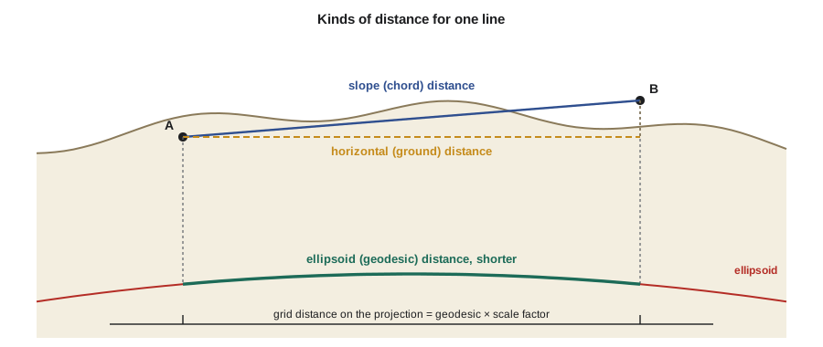
For a short line on a building site the differences are a few millimeters and often ignored. For a 2 km line at 900 m elevation, the ground and ellipsoid distances differ by about 28 cm, and the ellipsoid and grid distances by a further amount set by the projection. Lesson 9 of CIV-250 shows how the combined scale factor handles both. GNSS gives the chord, which a processing program converts to whatever distance is needed. The key habit is to label every distance by kind.
Measuring distance electronically
Steel tapes were the standard for centuries, and they still appear on small jobs, but most distances are now measured electronically. An electronic distance measurement (EDM) instrument sends modulated light to a reflector, or to the target surface itself in reflectorless mode, and measures either the phase difference between the outgoing and returning signal or the time of flight of a short pulse. Phase measurement compares the returning wave with the outgoing one at several modulation wavelengths to resolve the whole number of wavelengths; pulse measurement times the round trip with a very precise clock. Either way, the instrument must know the speed of light in the air along the line, which depends on temperature and pressure. A typical correction is about 1 part per million for every 1 °C of temperature or 3 hPa of pressure, so ignoring a 20 °C difference from the instrument's standard conditions would add about 20 mm to a 1 km line.
EDM accuracy is quoted as a constant plus a proportional part, for example ±(2 mm + 2 ppm). The constant part comes from centering, the reflector constant and the instrument's electronics; the proportional part comes mainly from the atmosphere. On a 500 m line, that specification gives \(\sqrt{2^2 + 1^2} \approx 2.2\) mm.
Angles, directions and their units
Total stations measure two kinds of angle. The horizontal angle is the angle in the horizontal plane between two directions. The vertical angle is measured from the horizontal upward or downward; most instruments actually report the zenith angle, measured from straight up, so that a horizontal line has a zenith angle of 90°. The vertical angle is 90° minus the zenith angle.
Directions are referred to a reference meridian. An azimuth is measured clockwise from north, from 0° to 360°. A bearing is measured from north or south toward east or west and never exceeds 90°, for example N 35°20′ E or S 12°05′ W. North itself has several meanings: true or geodetic north toward the pole, grid north along the projection's northing axis, and magnetic north toward the magnetic pole. The angle between true and grid north is the convergence, and the angle between true and magnetic north is the magnetic declination, which changes over time.
Degrees, minutes and seconds remain the standard in US surveying, and they appear in legal descriptions of property. Some software and European instruments use the gon or grad, in which a full circle is 400 gon, so a right angle is 100 gon. Mathematics and programming use radians, with \(2\pi\) in a circle. Military and some mapping applications use mils. Converting angles correctly is therefore a routine part of moving data between systems.
One useful rule of thumb links angles and distances: an angle of one second of arc subtends about 4.85 mm at 1 km. A total station whose angles are good to ±3″ can therefore place a point 300 m away to about ±4 mm in the direction across the line of sight.
Three ways to measure height
Heights are measured in three main ways, each with its own strengths.
Differential leveling uses a level that defines a horizontal line of sight and graduated rods held on the points. The difference in rod readings is the height difference. It is slow but very precise, about a millimeter per kilometer with care, and because the line of sight is perpendicular to gravity, it naturally produces orthometric height differences. National vertical networks were built this way.
Trigonometric heighting uses a total station: the height difference is the slope distance times the cosine of the zenith angle, plus the instrument height, minus the target height, with a correction for the Earth's curvature and atmospheric refraction over longer lines. It is faster than leveling and works across valleys and rivers, but it is less precise because refraction near the ground is hard to predict.
where \(S\) is the slope distance, \(z\) the zenith angle, \(h_i\) the instrument height, \(h_t\) the target height, \(R\) the Earth's radius and \(k\) the coefficient of refraction, often taken as about 0.13. The last term is about 6.8 cm over 1 km.
GNSS heighting measures ellipsoid heights, which become orthometric heights only after subtracting the geoid height from a geoid model, as explained in lesson 2. With a modern geoid model and good observations, GNSS can give elevations to a couple of centimeters, which is enough for most mapping and construction but not for precise leveling work such as long gravity sewers.
Worked problem
Trigonometric height across the Oldman River
For the bridge scour study, Grant sets the total station on a control point on the south bank of the Missouri River (instrument height 1.552 m) and sights a prism (target height 1.800 m) on the north bank. The slope distance is 612.384 m and the zenith angle is 91°12′40″. The control point's elevation is 1,005.214 m. Find the elevation of the prism point.
Show solution
- \[S\cos z = 612.384 \times \cos 91.2111° = -12.944\ \text{m}\]
- \[\text{curvature and refraction} = \frac{0.87 \times 612.384^2 \times \sin^2 91.2111°}{2 \times 6\,371\,000} = 0.026\ \text{m}\]
- \[\Delta H = -12.944 + 1.552 - 1.800 + 0.026 = -13.166\ \text{m}\]
- \[H = 1005.214 - 13.165 = 992.048\ \text{m}\]
Answer: The far-bank point is about 13.17 m lower. Because refraction over water can change during the day, the crew measures reciprocal observations from both banks at the same time and averages them, which cancels most of the curvature and refraction effect.
How errors carry through
Every observation has a random error, and the coordinates computed from observations inherit those errors. The law of propagation of variance tells us how. For a quantity computed as a function of several independent observations, the variance of the result is the sum of each observation's variance multiplied by the square of how sensitive the result is to that observation:
For the horizontal distance \(D = S\sin z\), errors in both \(S\) and \(z\) contribute, but for nearly horizontal lines the zenith angle contributes very little to \(D\) and a lot to the height difference. Thinking this way lets an engineer predict, before going to the field, whether a planned method can meet the required accuracy. Lesson 2 of CIV-250 works through these ideas in detail, and GEOM-220 Adjustment of Observations develops them into least squares, the standard method for combining redundant measurements.
Distances on the ellipsoid
For long lines, and for checking GNSS results, geomatics engineers compute distances and azimuths directly from latitudes and longitudes. On a sphere the haversine formula is simple and adequate for navigation. On the ellipsoid, the geodesic, the shortest path on the surface, is computed by iterative methods such as Vincenty's formulas or Karney's algorithm, which are accurate to well below a millimeter for lines of any length. The geodesic azimuth at each end is different, because meridians converge: on a long east–west line the forward and back azimuths differ by noticeably more than 180°.
# Geodesic distance and azimuths on GRS80 (Vincenty inverse) compared with a sphere
import math

a = 6378137.0
f = 1 / 298.257222101
b = a * (1 - f)

def vincenty(lat1, lon1, lat2, lon2):
    L = math.radians(lon2 - lon1)
    U1 = math.atan((1 - f) * math.tan(math.radians(lat1)))
    U2 = math.atan((1 - f) * math.tan(math.radians(lat2)))
    sU1, cU1, sU2, cU2 = math.sin(U1), math.cos(U1), math.sin(U2), math.cos(U2)
    lam = L
    for _ in range(200):
        sl, cl = math.sin(lam), math.cos(lam)
        ss = math.hypot(cU2 * sl, cU1 * sU2 - sU1 * cU2 * cl)
        cs = sU1 * sU2 + cU1 * cU2 * cl
        sig = math.atan2(ss, cs)
        sa = cU1 * cU2 * sl / ss
        c2a = 1 - sa * sa
        c2sm = cs - 2 * sU1 * sU2 / c2a
        C = f / 16 * c2a * (4 + f * (4 - 3 * c2a))
        prev = lam
        lam = L + (1 - C) * f * sa * (sig + C * ss * (c2sm + C * cs * (-1 + 2 * c2sm ** 2)))
        if abs(lam - prev) < 1e-12:
            break
    u2 = c2a * (a * a - b * b) / (b * b)
    A = 1 + u2 / 16384 * (4096 + u2 * (-768 + u2 * (320 - 175 * u2)))
    B = u2 / 1024 * (256 + u2 * (-128 + u2 * (74 - 47 * u2)))
    ds = B * ss * (c2sm + B / 4 * (cs * (-1 + 2 * c2sm ** 2)
         - B / 6 * c2sm * (-3 + 4 * ss ** 2) * (-3 + 4 * c2sm ** 2)))
    s = b * A * (sig - ds)
    az1 = math.degrees(math.atan2(cU2 * math.sin(lam), cU1 * sU2 - sU1 * cU2 * math.cos(lam))) % 360
    az2 = math.degrees(math.atan2(cU1 * math.sin(lam), -sU1 * cU2 + cU1 * sU2 * math.cos(lam))) % 360
    return s, az1, az2

def haversine(lat1, lon1, lat2, lon2, R=6371000.0):
    p1, p2 = math.radians(lat1), math.radians(lat2)
    dp, dl = p2 - p1, math.radians(lon2 - lon1)
    h = math.sin(dp / 2) ** 2 + math.cos(p1) * math.cos(p2) * math.sin(dl / 2) ** 2
    return 2 * R * math.asin(math.sqrt(h))

lines = {"Lethbridge to Great Falls": (49.6956, -112.8451, 47.5053, -111.3008),
         "Short site line": (49.697866, -112.835457, 49.700000, -112.828000)}
for name, (la1, lo1, la2, lo2) in lines.items():
    s, az1, az2 = vincenty(la1, lo1, la2, lo2)
    h = haversine(la1, lo1, la2, lo2)
    print(f"{name}: geodesic {s:,.3f} m, sphere {h:,.1f} m, difference {h - s:+,.1f} m")
    print(f"   forward azimuth {az1:.4f} deg, azimuth at far end {az2:.4f} deg")

# One arc-second at 1 km, and trigonometric heighting with curvature and refraction
print(f"1 arc-second at 1000 m = {1000 * math.radians(1 / 3600) * 1000:.2f} mm")
S, z = 612.384, math.radians(91 + 12 / 60 + 40 / 3600)
cr = (1 - 0.13) * (S * math.sin(z)) ** 2 / (2 * 6371000)
dH = S * math.cos(z) + 1.552 - 1.800 + cr
print(f"S cos z = {S * math.cos(z):.3f} m, c&r = {cr:.3f} m, dH = {dH:.3f} m")Lethbridge to Great Falls: geodesic 268,866.851 m, sphere 268,708.3 m, difference -158.5 m forward azimuth 154.3555 deg, azimuth at far end 155.5142 deg Short site line: geodesic 587.999 m, sphere 586.5 m, difference -1.5 m forward azimuth 66.1901 deg, azimuth at far end 66.1958 deg 1 arc-second at 1000 m = 4.85 mm S cos z = -12.944 m, c&r = 0.026 m, dH = -13.166 m
The sphere is wrong by about 158 m over the 269 km line between the two cities, roughly 0.06 percent, and even on the 588 m site line it is 1.5 m short, because a mean radius of 6,371 km does not match the ellipsoid's curvature at these latitudes. That is far too large for surveying, although it is fine for estimating flight distances. The azimuth of the long line turns by more than a degree between its two ends: the direction of travel at Great Falls is about 1.16° larger than at Lethbridge, so the back azimuth is not simply the forward azimuth plus 180°. On the site line the change is only 20 seconds. This turning is the meridian convergence described in lesson 3. The final lines reproduce the river crossing example, rounded to the millimeter.
Common mistakes
MistakeUsing a slope distance where a horizontal, ellipsoid or grid distance is needed.
InsteadLabel every distance by kind and reduce it deliberately.
MistakeTreating a bearing as an azimuth or mixing true, grid and magnetic north.
InsteadState the reference meridian and convert carefully; apply convergence and declination.
MistakeIgnoring curvature and refraction on long trigonometric sights.
InsteadApply the correction, or use simultaneous reciprocal observations.
MistakeUsing GNSS ellipsoid heights as elevations.
InsteadSubtract the geoid height from an official geoid model.
Summary and key terms
- Slope, horizontal, ellipsoid, grid and chord distances are different quantities.
- EDM accuracy is a constant plus parts per million, and depends on correcting for the atmosphere.
- Azimuths run 0–360° clockwise from north; bearings are quadrant angles up to 90°.
- One arc-second subtends about 4.85 mm at 1 km.
- Heights come from leveling, trigonometric heighting or GNSS with a geoid model.
- The law of propagation of variance predicts how observation errors affect computed results.
- Slope distance
- The straight-line distance between instrument and target.
- Zenith angle
- A vertical angle measured downward from straight up.
- Azimuth
- A direction measured clockwise from north, from 0° to 360°.
- Bearing
- A direction given as an angle up to 90° east or west of north or south.
- Magnetic declination
- The angle between true north and magnetic north at a place and time.
- Geodesic
- The shortest path between two points on the ellipsoid.
- Propagation of variance
- The rule for computing the uncertainty of a result from the uncertainties of the observations.
Practice problems
Work each problem on paper first, then reveal the answer to check.
Convert an azimuth of 214°30′ to a bearing.
Show answer
S 34°30′ W.
An EDM is rated ±(3 mm + 2 ppm). Estimate its standard error on a 1.5 km line.
Show answer
\(\sqrt{3^2 + 3^2} \approx 4.2\) mm.
What lateral offset does a 5″ angle error cause at 400 m?
Show answer
\(400 \times 5 \times 4.848\times10^{-6} = 9.7\) mm.
Compute the curvature and refraction correction for a 2 km horizontal sight with k = 0.13.
Show answer
\(0.87 \times 2000^2/(2 \times 6\,371\,000) = 0.273\) m.
Why are reciprocal observations used across a river?
Show answer
Measuring from both ends at the same time cancels most of the curvature and refraction effect.
Lesson quiz · 5 questions
Score 60% or more to complete this lesson.
Create a free account to save your progress, take quizzes and earn a certificate.