
CMPUT-411 · Lesson 9 of 12 · 38 min
Texturing and mapping
Geometry alone gives shape; textures give surfaces their detail. A texture is an image, or a function, sampled across a surface to vary color, roughness, normals, displacement or any other shading input from point to point. Edwin Catmull introduced texture mapping in his 1974 thesis at the University of Utah, and James Blinn and Martin Newell added environment mapping in 1976 and bump mapping in 1978. Today a single object in a game may carry half a dozen texture maps, and textures account for most of the memory a renderer uses. This lesson covers how surfaces are parameterized, how textures are addressed and interpolated, how filtering and mipmaps prevent aliasing, and the main kinds of maps: normal and displacement maps, environment maps and procedural textures.
Texture coordinates and parameterization
To map an image onto a surface, every point on the surface needs coordinates in the image, conventionally called \((u, v)\) and ranging from 0 to 1 across the texture. For a mesh, artists or tools assign \((u, v)\) to each vertex, and the rasterizer interpolates them across each triangle. Assigning these coordinates is called UV mapping or unwrapping: cutting the surface along seams and flattening the pieces, called charts or islands, into the unit square, much as a tailor's pattern flattens a jacket. A planet or a soda can has a natural parameterization (spherical or cylindrical coordinates); a character's head does not.
Every flattening of a curved surface introduces distortion, a consequence of Gauss's Theorema Egregium: a sphere cannot be mapped to a plane without stretching. Unwrapping algorithms therefore trade off angle distortion (conformal maps such as least-squares conformal mapping, 2002, preserve angles locally) against area distortion, and against the number and placement of seams, which can cause visible discontinuities. Texel density, the number of texels per unit of surface area, should be roughly uniform so that detail does not blur in one region and waste memory in another. Atlases pack many charts, often from many objects, into one texture to reduce state changes on the GPU. A different approach, Disney's Ptex (2008), stores a separate small texture per mesh face and avoids explicit UV unwrapping altogether; it is common in film but not in real-time engines.
Texture coordinates outside \([0, 1]\) are handled by the addressing or wrap mode. Repeat (wrap) mode takes the fractional part, tiling the texture, which is how a small brick image covers a long wall. Mirrored repeat flips every other tile to hide seams. Clamp-to-edge repeats the border texels, which suits decals and screen-space effects. Clamp-to-border returns a fixed color. Choosing the wrong mode produces seams or smeared edges.
Perspective-correct interpolation
Lesson 2 interpolated attributes across a triangle with barycentric coordinates computed in screen space. That is wrong for perspective projections. Equal steps across the screen do not correspond to equal steps across the triangle in 3D: the far end of a receding floor is compressed on screen. Interpolating \((u, v)\) linearly in screen space, called affine texture mapping, makes textures appear to swim and bend along triangle diagonals, an artifact familiar from the original PlayStation (1994), which lacked perspective correction.
The correct method rests on a fact from lesson 5: after projection, quantities divided by the clip-space w (proportional to eye-space depth) vary linearly in screen space. The rasterizer therefore interpolates \(u/w\), \(v/w\) and \(1/w\) linearly, and at each pixel divides to recover \(u = (u/w)/(1/w)\). Modern GPUs perform this perspective-correct interpolation for every varying attribute automatically, unless a shader asks for screen-space (noperspective) interpolation.
# Why texture coordinates must be interpolated with perspective correction.
# A floor quad recedes from the camera; we interpolate u along one scanline
# in screen space (affine) and with the 1/w method, and compare with the truth.
import numpy as np
# two vertices of an edge: near (w = 1) and far (w = 5), with u = 0 and u = 1
w0, w1 = 1.0, 5.0
u0, u1 = 0.0, 1.0
print(" screen t   affine u   perspective-correct u   true u")
for t in (0.0, 0.25, 0.5, 0.75, 1.0):
    affine = (1 - t) * u0 + t * u1
    # interpolate u/w and 1/w linearly in screen space, then divide
    num = (1 - t) * u0 / w0 + t * u1 / w1
    den = (1 - t) / w0 + t / w1
    correct = num / den
    # ground truth: the point at screen fraction t lies at eye-space depth z with
    # 1/z linear in t; recover the world fraction along the edge
    z = 1 / den
    true = (z - w0) / (w1 - w0)
print(f"{t:9.2f} {affine:8.3f} {correct:21.3f} {true:6.3f}") screen t affine u perspective-correct u true u
0.00 0.000 0.000 0.000
0.25 0.250 0.062 0.062
0.50 0.500 0.167 0.167
0.75 0.750 0.375 0.375
1.00 1.000 1.000 1.000Halfway across the screen, affine interpolation reports \(u = 0.5\), but the true point on the edge is only about a sixth of the way along, because the near half of the edge occupies most of the screen. The perspective-correct formula matches the ground truth exactly at every sample.
Sampling textures: magnification and minification
When a texture is displayed, each screen pixel must be assigned a value from the texture, and pixels and texels almost never line up. Two cases arise. In magnification, one texel covers several pixels, as when the camera is close to a wall; the question is how to fill in values between texel centers. In minification, one pixel covers many texels, as on a distant or steeply tilted surface; then the texture contains detail finer than the pixel grid can represent, and sampling it at one point per pixel aliases, producing shimmering and moiré patterns, exactly the problem of lesson 2.
For magnification, nearest-neighbor filtering returns the texel containing the sample point, which looks blocky, a look sometimes chosen deliberately for pixel art. Bilinear filtering takes the four nearest texel centers and blends them with weights from the fractional position, first along u and then along v. It produces smooth gradients but blurs sharp edges when magnified a lot. Bicubic filtering uses a 4 × 4 neighborhood for smoother results at higher cost.
# Nearest-texel versus bilinear filtering of a tiny 4 x 4 texture,
# sampled at a few texture coordinates (u, v in [0, 1], texel middles at
# (i + 0.5) / 4).
import numpy as np
tex = np.array([[0, 0, 255, 255],
                [0, 0, 255, 255],
                [64, 64, 128, 128],
                [64, 64, 128, 128]], dtype=float)
N = 4
def nearest(u, v):
    i = min(int(u * N), N - 1); j = min(int(v * N), N - 1)
    return tex[j, i]
def bilinear(u, v):
    x = u * N - 0.5; y = v * N - 0.5                # continuous texel coordinates
    x0 = int(np.floor(x)); y0 = int(np.floor(y)); fx = x - x0; fy = y - y0
    def t(i, j):                                    # clamp-to-edge addressing
        return tex[min(max(j, 0), N - 1), min(max(i, 0), N - 1)]
    top = (1 - fx) * t(x0, y0) + fx * t(x0 + 1, y0)
    bot = (1 - fx) * t(x0, y0 + 1) + fx * t(x0 + 1, y0 + 1)
    return (1 - fy) * top + fy * bot
for u, v in [(0.125, 0.125), (0.45, 0.125), (0.5, 0.125), (0.55, 0.125), (0.5, 0.5), (0.9, 0.9)]:
print(f"u={u:5.3f} v={v:5.3f} nearest {nearest(u, v):6.1f} bilinear {bilinear(u, v):6.1f}")u=0.125 v=0.125 nearest 0.0 bilinear 0.0 u=0.450 v=0.125 nearest 0.0 bilinear 76.5 u=0.500 v=0.125 nearest 255.0 bilinear 127.5 u=0.550 v=0.125 nearest 255.0 bilinear 178.5 u=0.500 v=0.500 nearest 128.0 bilinear 111.8 u=0.900 v=0.900 nearest 128.0 bilinear 128.0
Near the sharp boundary between the black and white columns, nearest-neighbor jumps from 0 to 255, while bilinear ramps across it: at u = 0.5, exactly on the edge between texel centers, it returns the average, 127.5. At the center of the texture the bilinear value mixes all four quadrants. Exactly at a texel center, such as (0.125, 0.125), both filters agree.
Mipmaps and trilinear filtering
Minification needs prefiltering: averaging the many texels a pixel covers before sampling. Computing that average per pixel at run time would be too slow, so Lance Williams's 1983 mipmapping precomputes it. A mipmap (from the Latin multum in parvo, 'much in a small place') is a chain of images, each half the width and height of the previous one, down to 1 × 1, with each level made by low-pass filtering the one above, typically with a box or Kaiser filter. The whole chain costs only a third more memory than the base level, because \(1 + 1/4 + 1/16 + \dots = 4/3\).
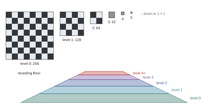
At render time the GPU estimates how many texels a pixel covers from the screen-space derivatives of the texture coordinates, \(\partial u/\partial x\), \(\partial v/\partial x\), \(\partial u/\partial y\) and \(\partial v/\partial y\), which it obtains cheaply by differencing values between neighboring pixels in each 2 × 2 quad of fragments (lesson 6). The level of detail is \(\lambda = \log_2 \rho\), where \(\rho\) is the larger of the two footprint lengths in texels. Level 0 is used for \(\lambda \le 0\) (magnification). Trilinear filtering performs bilinear lookups in the two nearest levels and blends them by the fractional part of \(\lambda\), avoiding visible bands where the level changes.
# Building a mipmap chain for a 256 x 256 texture and choosing the level of
# detail from screen-space derivatives of the texture coordinates.
import math
size = 256
levels = []
s = size
while s >= 1:
    levels.append(s); s //= 2
print("mip levels:", levels)
base = size * size
total = sum(l * l for l in levels)
print(f"memory of full chain / base level = {total / base:.4f}  (about 4/3)")
# level of detail: rho = texels covered per pixel along the larger axis
def lod(du_dx, dv_dx, du_dy, dv_dy):
    rx = math.hypot(du_dx * size, dv_dx * size)
    ry = math.hypot(du_dy * size, dv_dy * size)
    rho = max(rx, ry)
    return max(0.0, math.log2(rho)), rho
for name, d in [("texture magnified (close-up)", (0.5 / size, 0, 0, 0.5 / size)),
                ("one texel per pixel", (1 / size, 0, 0, 1 / size)),
                ("4 texels per pixel", (4 / size, 0, 0, 4 / size)),
                ("floor at grazing angle", (1 / size, 0, 0, 24 / size))]:
    L, rho = lod(*d)
print(f"{name:30} rho = {rho:5.1f} LOD = {L:4.2f} -> blend levels {int(L)} and {int(L) + 1 if L > 0 else 0}")mip levels: [256, 128, 64, 32, 16, 8, 4, 2, 1] memory of full chain / base level = 1.3333 (about 4/3) texture magnified (close-up) rho = 0.5 LOD = 0.00 -> blend levels 0 and 0 one texel per pixel rho = 1.0 LOD = 0.00 -> blend levels 0 and 0 4 texels per pixel rho = 4.0 LOD = 2.00 -> blend levels 2 and 3 floor at grazing angle rho = 24.0 LOD = 4.58 -> blend levels 4 and 5
The last line exposes mipmapping's weakness. On a floor seen at a grazing angle, a pixel's footprint is long and thin: one texel across but 24 along the view direction. Isotropic mipmapping must choose a single level from the longer axis, so it picks level 4.6 and blurs the floor in both directions, although detail across the view direction could have been kept. Anisotropic filtering solves this by taking several trilinear samples along the long axis of the footprint at a finer level; GPUs support up to 16 samples, and the setting is one of the best-value quality options in games. Summed-area tables (Franklin Crow, 1984) are another prefiltering method that supports rectangular footprints, but they use more memory and are rarely used for color textures.
Filtering assumes texture values can be averaged. That holds for color stored linearly (sRGB textures are decoded to linear before filtering, as lesson 1 explained) but not for normals, whose average shortens and loses orientation detail, or for roughness, where averaging bumps should increase effective roughness. Techniques such as LEAN mapping (2010) and Toksvig's normal-map adjustment (2005) adjust roughness in lower mip levels to account for this, reducing sparkling highlights on distant surfaces.
Texture compression and storage
Uncompressed textures are large: a 4096 × 4096 RGBA texture with 8 bits per channel takes 64 MB, plus a third more for mipmaps. GPUs therefore support block-compressed formats that the hardware decodes on the fly during sampling, so textures stay compressed in memory. Formats split the image into 4 × 4 blocks and store each block in a fixed number of bits, which allows random access. The BC (block compression) family on desktop GPUs includes BC1 at 4 bits per texel for color, BC5 for two-channel normal maps, BC6H for HDR and BC7 for high-quality color at 8 bits per texel. Mobile GPUs use ETC2 and ASTC, which supports block sizes from 4 × 4 to 12 × 12 for a choice of quality and size. These formats are lossy and asymmetric: encoding is slow and done offline, decoding is fast. Virtual texturing (megatextures), used in id Software's Rage (2011) and in Unreal Engine's virtual textures, streams only the tiles visible at the needed resolution, allowing texture data far larger than GPU memory.
| Format | Bits per texel | Typical use |
|---|---|---|
| RGBA8 (uncompressed) | 32 | Render targets, small UI textures |
| BC1 | 4 | Opaque color with low quality demands |
| BC3 | 8 | Color with smooth alpha |
| BC5 | 8 | Tangent-space normal maps (two channels) |
| BC6H | 8 | HDR environment maps and lightmaps |
| BC7 | 8 | High-quality color and alpha |
| ASTC 4×4 to 12×12 | 8 down to 0.89 | Mobile and some desktop GPUs; flexible quality |
Normal, bump and displacement maps
Textures can perturb geometry as well as color. Blinn's bump mapping (1978) perturbs the shading normal using the derivatives of a height map, so a smooth surface shades as if it were rough, without changing its silhouette. Normal mapping, its modern form, stores the perturbed normal directly in a texture's RGB channels, mapped from \([-1, 1]\) to \([0, 1]\). Tangent-space normal maps express the normal relative to a per-vertex frame of tangent, bitangent and normal (TBN); their dominant blue color comes from the unperturbed normal (0, 0, 1). Because they are relative to the surface, they can be reused across deforming and tiled meshes. A common workflow bakes the fine detail of a sculpted multi-million-polygon model into a normal map for a low-polygon game model, so a character can show pores and stitching on a few thousand triangles.
Normal maps change only shading. Parallax mapping offsets the texture lookup by the view direction and a height map to fake depth, and parallax occlusion mapping ray-marches the height field per pixel, giving convincing bricks and cobblestones that occlude each other, though silhouettes stay flat. True displacement mapping moves vertices, usually after tessellating the surface finely (lesson 7), changing silhouettes and shadows; offline renderers have long subdivided to micropolygons for this, as Pixar's RenderMan did from the Reyes architecture of 1987 onward, and modern engines use hardware tessellation or, in Unreal Engine 5, the Nanite virtualized geometry system (2021) to render geometry detailed enough that displacement becomes ordinary geometry.
Environment and reflection mapping
Environment mapping approximates reflections of a distant surrounding scene by looking up a texture indexed by direction. Blinn and Newell's 1976 version used a latitude-longitude map; sphere maps (a photograph of a mirrored ball) followed; cube maps, six square textures forming the faces of a cube around the viewer, are now universal because they have little distortion and GPUs support them directly. A reflective surface computes the reflected view direction \(r = 2(n \cdot v)n - v\) and samples the cube map in that direction. Because the environment is assumed infinitely far away, reflections of nearby objects are wrong; parallax-corrected cube maps and reflection probes placed around a level reduce the error, and screen-space reflections or ray tracing handle nearby geometry. As lesson 8 explained, HDR environment maps prefiltered for each roughness level also provide image-based lighting for physically based materials.
Procedural textures and noise
Instead of storing an image, a procedural texture computes its value from a function of position, which gives unlimited resolution, no seams, tiny storage and the ability to texture solids (wood grain or marble that runs through an object, which Darwyn Peachey and Ken Perlin both showed in 1985). Ken Perlin's noise function, which he developed after working on the film Tron (1982) and published in 1985, and for which he received a Technical Achievement Academy Award in 1997, is the basis of most procedural texturing. It is a smooth, pseudo-random function with a known frequency: random gradients are placed at integer lattice points, and the value between them blends the gradient ramps with a smooth fade curve. Perlin's improved noise (2002) replaced the cubic fade \(3t^2 - 2t^3\) with the quintic \(6t^5 - 15t^4 + 10t^3\), whose second derivative is continuous. Simplex noise (2001) uses a simplex lattice for lower cost in higher dimensions.
Summing noise at doubling frequencies and halving amplitudes, called fractional Brownian motion (fBm) or turbulence, produces the multi-scale detail of clouds, terrain, rust and marble. Worley's cellular noise (1996) gives cell-like patterns for stone, scales and crackle. Procedural textures are central to film rendering and to tools such as Substance Designer, Blender and Houdini, though games usually bake them into image textures because sampling an image is cheaper than evaluating noise per pixel and filtering procedural functions is hard.
# One-dimensional gradient noise in the style of Perlin (1985/2002), with the
# quintic fade curve, plus a fractal sum of octaves (fBm). Each is printed as a
# strip whose character density shows the value, and we measure roughness as the
# mean jump between adjacent samples.
import random, math
random.seed(411)
grad = [random.uniform(-1, 1) for _ in range(256)]
perm = list(range(256)); random.shuffle(perm)
def fade(t): return t * t * t * (t * (t * 6 - 15) + 10)
def noise(x):
    i = math.floor(x); f = x - i
    g0 = grad[perm[i & 255]]; g1 = grad[perm[(i + 1) & 255]]
    return (1 - fade(f)) * g0 * f + fade(f) * g1 * (f - 1)   # blend the two ramps
def fbm(x, octaves=5):
    total, amp, freq = 0.0, 1.0, 1.0
    for _ in range(octaves):
        total += amp * noise(x * freq); amp *= 0.5; freq *= 2.03   # not exactly 2, to avoid aligned lattices
    return total
ramp = " .:-=+*#%@"
xs = [k * 0.1 for k in range(64)]
for name, fn in (("noise", noise), ("fBm", fbm)):
    vals = [fn(x) for x in xs]
    lo, hi = min(vals), max(vals)
    strip = "".join(ramp[min(int((v - lo) / (hi - lo) * len(ramp)), len(ramp) - 1)] for v in vals)
    rough = sum(abs(vals[i + 1] - vals[i]) for i in range(len(vals) - 1)) / (len(vals) - 1)
    print(f"{name:5} |{strip}|  range {lo:+.2f}..{hi:+.2f}  mean jump {rough:.3f}")
print("noise at integer lattice points:", [abs(round(noise(k), 6)) for k in range(5)])noise |=-----=====-:. .-=+#%@@@%*+=-::::--===--:. .:=+***+=---=++*| range -0.18..+0.24 mean jump 0.030 fBm |-::-:-=::--=+=. :---=+#@@#+===:-.:-=*=-:.. . .:+#***+::::++=+| range -0.22..+0.32 mean jump 0.058 noise at integer lattice points: [0.0, 0.0, 0.0, 0.0, 0.0]
In each strip, denser characters mean higher values. The plain noise strip changes gradually, with features about one lattice cell (ten samples) wide, and it is exactly zero at the integer lattice points, a property of gradient noise. The fBm strip keeps the same large-scale shape but adds finer variation from the higher octaves, which shows up as a larger mean jump between neighboring samples. The octave frequencies are multiplied by 2.03 rather than exactly 2 so that the lattices of different octaves do not line up, a common trick to avoid visible regularity. Changing the seed gives a different but statistically identical texture, which is how terrain generators make endless landscapes.
Texturing in practice
A modern physically based material is a set of aligned texture maps: base color (sRGB), metallic and roughness (often packed into channels of one linear texture), a tangent-space normal map, ambient occlusion and sometimes height, emission and opacity. glTF 2.0, the Khronos 'JPEG of 3D' standard published in 2017, defines exactly this set and is widely used on the web and in pipelines. Artists author textures in tools such as Adobe Substance 3D Painter and Designer, Blender and Mari, or capture them with photogrammetry and material scanners. Texture streaming loads mip levels on demand as the camera moves, and texture budgets are a major constraint on console and mobile memory.
Worked examples
Worked problem
Perspective-correct midpoint
An edge has u = 0 at a vertex with w = 2 and u = 1 at a vertex with w = 6. What u should the pixel halfway between them on screen receive?
Show solution
- Interpolate u/w: \(0.5 \times 0/2 + 0.5 \times 1/6 = 0.0833\).
- Interpolate 1/w: \(0.5 \times 1/2 + 0.5 \times 1/6 = 0.3333\).
- Divide: \(u = 0.0833 / 0.3333 = 0.25\).
Answer: u = 0.25, not the affine value 0.5: the near half of the edge fills most of the screen.
Worked problem
Mipmap level
A 1024 × 1024 texture is drawn so that one screen pixel spans 3 texels horizontally and 12 texels vertically. Which mip level does isotropic trilinear filtering use, and what does anisotropic filtering do differently?
Show solution
- \(\rho = \max(3, 12) = 12\), so \(\lambda = \log_2 12 = 3.58\).
- Trilinear filtering blends levels 3 (128 × 128) and 4 (64 × 64), weighting level 4 by 0.58.
- Anisotropic filtering uses the shorter axis, \(\log_2 3 = 1.58\), and takes about four samples (12/3) along the long axis.
Answer: Level 3.58 for trilinear; anisotropic filtering samples near level 1.58 along the footprint, keeping more detail.
Worked problem
Memory budget
How much memory does a 2048 × 2048 texture with a full mip chain need uncompressed (RGBA8) and in BC7?
Show solution
- Base level: \(2048^2 = 4{,}194{,}304\) texels.
- RGBA8: \(4 \times 4.19 = 16.8\) MB; with mips \(\times 4/3 = 22.4\) MB.
- BC7 at 1 byte per texel: \(4.19 \times 4/3 = 5.6\) MB.
Answer: About 22.4 MB uncompressed and 5.6 MB in BC7, a fourfold saving.
Common mistakes
MistakeInterpolate texture coordinates linearly in screen space under perspective.
InsteadInterpolate u/w and 1/w and divide; GPUs do this by default.
MistakeSample minified textures without mipmaps.
InsteadUse mipmaps with trilinear, and preferably anisotropic, filtering to avoid shimmering.
MistakeFilter sRGB color values directly.
InsteadDecode to linear before filtering and blending.
MistakeStore normal maps in sRGB or compress them like color.
InsteadStore normals as linear data and use a two-channel format such as BC5.
MistakeAssume a normal map changes silhouettes.
InsteadNormal and parallax maps change shading only; use displacement or real geometry for silhouettes.
Summary and key terms
- Texture coordinates (u, v) map surface points to a texture; unwrapping a curved surface always introduces distortion and seams.
- Wrap modes (repeat, mirror, clamp) define lookups outside [0, 1].
- Perspective-correct interpolation divides interpolated u/w by interpolated 1/w.
- Bilinear filtering handles magnification; mipmaps with trilinear filtering prefilter minification at a 4/3 memory cost.
- Anisotropic filtering preserves detail on surfaces seen at grazing angles.
- Block-compressed formats such as BC7 and ASTC keep textures compressed in GPU memory.
- Normal, parallax and displacement maps add surface detail at increasing cost; environment maps approximate distant reflections.
- Procedural textures built from gradient noise and fBm give unlimited resolution with tiny storage.
- Texture mapping
- Varying shading inputs across a surface by sampling an image or function at texture coordinates.
- UV unwrapping
- Flattening a surface into charts in texture space to assign texture coordinates.
- Perspective-correct interpolation
- Interpolating attributes divided by w, then dividing by interpolated 1/w.
- Bilinear filtering
- Blending the four nearest texels according to the sample position.
- Mipmap
- A chain of prefiltered texture images, each half the resolution of the previous.
- Trilinear filtering
- Blending bilinear samples from two adjacent mip levels.
- Anisotropic filtering
- Taking several samples along the long axis of a pixel footprint in texture space.
- Normal map
- A texture storing perturbed surface normals for shading.
- Cube map
- Six textures forming a cube, indexed by direction, used for environments and reflections.
- Gradient noise
- A smooth pseudo-random function built from random gradients at lattice points.
Practice problems
Work each problem on paper first, then reveal the answer to check.
What wrap mode tiles a texture across a large surface?
Show answer
Repeat (wrap).
Why do affine-mapped textures appear to swim?
Show answer
Linear screen-space interpolation ignores perspective foreshortening.
Which three quantities does the rasterizer interpolate for perspective-correct u?
Show answer
u/w, 1/w (and v/w for v).
How much extra memory does a full mip chain need?
Show answer
About one third of the base level.
What is the level of detail when a pixel covers 8 texels?
Show answer
\(\log_2 8 = 3\).
Why does isotropic mipmapping blur floors at grazing angles?
Show answer
It must choose a level from the longest axis of a long, thin footprint.
Why are tangent-space normal maps mostly blue?
Show answer
The unperturbed normal (0, 0, 1) maps to RGB (0.5, 0.5, 1).
What does parallax occlusion mapping not change?
Show answer
The silhouette of the object.
What reflected direction is used to sample an environment map?
Show answer
\(r = 2(n \cdot v)n - v\).
What does fBm add to plain noise?
Show answer
Finer detail from summed octaves at doubling frequency and halving amplitude.
Lesson quiz · 5 questions
Score 60% or more to complete this lesson.
Create a free account to save your progress, take quizzes and earn a certificate.