
CMPUT-411 · Lesson 3 of 12 · 34 min
Transformations and homogeneous coordinates
Every object in a rendered scene is positioned, oriented and sized by transformations. A model of a chair is built once in its own coordinates and then placed in a room by a transformation; the room is seen through a camera by another; the camera's view is projected onto the screen by a third. Transformations are linear algebra applied to geometry, and this lesson assumes the matrix algebra and linear transformations of MATH-125 (lessons 4 and 8). ROB-210 develops rotations and rigid-body transforms for robot arms (lessons 2 to 4); here we focus on how graphics uses them: homogeneous coordinates, the order of composition, transforming normals correctly, and organizing transforms in a scene graph.
Linear and affine transformations
A linear transformation maps vectors by a matrix: \(x' = Mx\). In two dimensions, scaling by \(s_x, s_y\), rotation by an angle \(\theta\) about the origin, shear and reflection are all linear. Linear transformations keep the origin fixed and map lines to lines and parallel lines to parallel lines. Translation, moving every point by an offset \(t\), is not linear, because it moves the origin. Transformations of the form \(x' = Mx + t\), a linear map followed by a translation, are called affine. Affine maps preserve straight lines, parallelism and ratios of distances along a line, but not necessarily lengths or angles.
| Transformation | 2D matrix (linear part) | Preserves |
|---|---|---|
| Uniform scale by s | \(\begin{bmatrix} s & 0 \\ 0 & s \end{bmatrix}\) | Angles, shape (similarity) |
| Non-uniform scale | \(\begin{bmatrix} s_x & 0 \\ 0 & s_y \end{bmatrix}\) | Parallel lines, axis directions |
| Rotation by θ | \(\begin{bmatrix} \cos\theta & -\sin\theta \\ \sin\theta & \cos\theta \end{bmatrix}\) | Lengths, angles, handedness |
| Shear in x by k | \(\begin{bmatrix} 1 & k \\ 0 & 1 \end{bmatrix}\) | Area, parallel lines |
| Reflection in the y axis | \(\begin{bmatrix} -1 & 0 \\ 0 & 1 \end{bmatrix}\) | Lengths and angles; reverses handedness |
A rigid transformation, or rigid-body motion, combines rotation and translation and preserves all distances and angles; it moves objects without deforming them. A similarity adds uniform scaling. These categories matter in practice: rigid transforms can be inverted cheaply, similarities keep normals pointing the right way after renormalization, and general affine maps with non-uniform scale or shear need the special treatment of normals discussed below.
Homogeneous coordinates
It would be convenient if translation, like rotation and scale, were a matrix multiplication, so that any sequence of transformations could be combined into one matrix. Homogeneous coordinates achieve this by adding one coordinate. A 2D point \((x, y)\) is written \((x, y, 1)\) and a 3D point \((x, y, z, 1)\). An affine transformation then becomes a single matrix with the linear part in the upper-left block and the translation in the last column:
In 3D the matrices are 4 by 4, which is why GPU shading languages have built-in vec4 and mat4 types. The fourth coordinate w distinguishes points from directions. Points have \(w = 1\) and are affected by translation; directions, such as surface normals, light directions and velocities, have \(w = 0\), so the translation column multiplies zero and has no effect. This matches geometry: moving an object does not change which way its surfaces face. Differences of points (\(w = 1 - 1 = 0\)) are directions, and sums of points are meaningful only as weighted averages whose weights sum to one, such as barycentric combinations.
Homogeneous coordinates have a deeper meaning from projective geometry: the vector \((x, y, z, w)\) with \(w \ne 0\) represents the same point as \((x/w, y/w, z/w, 1)\), so all non-zero multiples are equivalent. This lets a 4 by 4 matrix express perspective projection, in which the final w depends on depth, and the division by w performs the perspective foreshortening. Lesson 5 uses this. Points with \(w = 0\) can be read as points at infinity in a given direction, which is how directional lights such as the sun are represented.
Composing transformations
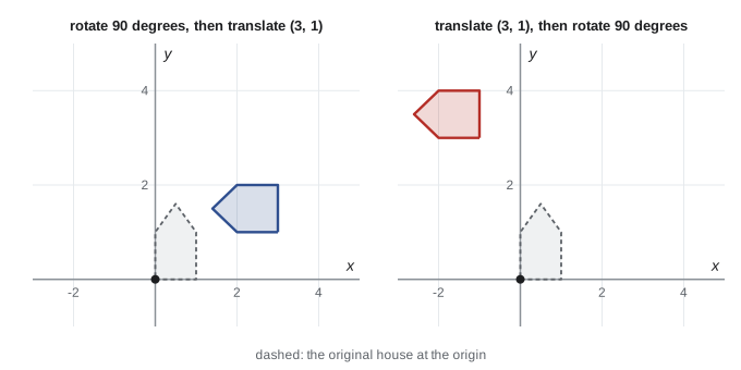
With column vectors, as used in this course and in OpenGL conventions, a transformation applied to a point is \(Mp\), and applying \(A\) then \(B\) gives \(B(Ap) = (BA)p\). The matrix nearest the vector acts first. Matrix multiplication is associative, so any chain can be precomputed into a single matrix, which is what makes homogeneous coordinates so useful: a renderer multiplies each vertex by one combined matrix instead of applying a dozen transformations in turn. But matrix multiplication is not commutative, so order matters. Rotating a point and then translating it is not the same as translating it and then rotating, because the rotation is always about the origin of the current coordinate frame.
# Homogeneous 2D transforms: composition order matters, and inverses undo.
import numpy as np
np.set_printoptions(precision=3, suppress=True)
def T(tx, ty): return np.array([[1, 0, tx], [0, 1, ty], [0, 0, 1]], float)
def R(deg):
    c, s = np.cos(np.radians(deg)), np.sin(np.radians(deg))
    return np.array([[c, -s, 0], [s, c, 0], [0, 0, 1]])
def S(sx, sy): return np.array([[sx, 0, 0], [0, sy, 0], [0, 0, 1]], float)
p = np.array([1.0, 0.0, 1.0])                 # a point (w = 1)
v = np.array([1.0, 0.0, 0.0])                 # a direction (w = 0)
A = T(3, 1) @ R(90)                           # rotate first, then translate
B = R(90) @ T(3, 1)                           # translate first, then rotate
print("rotate then translate:", (A @ p)[:2], "  translate then rotate:", (B @ p)[:2])
print("a direction ignores translation:", (A @ v)[:2])
# Rotate 90 degrees about the pivot (2, 2) rather than the origin
pivot = T(2, 2) @ R(90) @ T(-2, -2)
print("corner (3, 2) about pivot (2, 2) ->", (pivot @ np.array([3, 2, 1.0]))[:2])
M = T(4, -1) @ R(30) @ S(2, 0.5)               # a general affine transform
Minv = np.linalg.inv(M)
alt = S(0.5, 2) @ R(-30) @ T(-4, 1)            # inverse = reversed product of inverses
print("inverse matches reversed product of inverses:", np.allclose(Minv, alt))
print("M @ Minv =\n", np.round(M @ Minv, 6) + 0.0)rotate then translate: [3. 2.] translate then rotate: [-1. 4.] a direction ignores translation: [0. 1.] corner (3, 2) about pivot (2, 2) -> [2. 3.] inverse matches reversed product of inverses: True M @ Minv = [[1. 0. 0.] [0. 1. 0.] [0. 0. 1.]]
The program confirms the figure. The point (1, 0) rotated by 90 degrees becomes (0, 1); translating then gives (3, 2). Translating first gives (4, 1), which the rotation swings to (−1, 4). The direction vector, with w = 0, is rotated but not translated. To rotate about a point other than the origin, the standard idiom is to translate the pivot to the origin, rotate, and translate back: \(T(c)\,R\,T(-c)\). The same sandwich pattern scales an object about its center.
Inverting transformations is equally common: the camera's view matrix is the inverse of the matrix that places the camera in the world, and picking an object with the mouse requires mapping screen points back to world space. The inverse of a product is the product of the inverses in reverse order, \((ABC)^{-1} = C^{-1}B^{-1}A^{-1}\), and for each basic transformation the inverse is simple: translate by the negative offset, rotate by the negative angle, scale by the reciprocal. For a rigid transform with rotation \(R\) and translation \(t\), the inverse is rotation \(R^T\) and translation \(-R^T t\), since a rotation matrix is orthogonal (\(R^{-1} = R^T\)). Using this instead of a general matrix inverse is faster and numerically better.
Row-vector conventions, used by Direct3D's traditional mathematics libraries and many game engines, write points as rows and multiply \(pM\), so the leftmost matrix acts first and every matrix is the transpose of its column-vector counterpart. Both conventions are correct, and both appear in practice; mixing them is a frequent source of bugs, as is confusing the memory layout of a matrix (row-major or column-major) with the mathematical convention. When code produces a mirrored or exploded scene, a transposed matrix is the first suspect.
Transforming normals
Vertices, directions and normals do not all transform the same way. A surface normal is defined by being perpendicular to the surface: for any tangent vector \(t\) lying in the surface, \(n \cdot t = 0\), or \(n^T t = 0\). If the surface is transformed by \(M\), tangents transform as \(t' = Mt\), because they are differences of points on the surface. We want a matrix \(G\) such that \(n' = Gn\) stays perpendicular: \(n'^T t' = n^T G^T M t = 0\) for all tangents. This holds if \(G^T M = I\), so \(G = (M^{-1})^T\), the inverse transpose of the linear part of \(M\).
# Why normals transform by the inverse transpose. A surface tangent t and its
# normal n are perpendicular; a non-uniform scale preserves that only if the
# normal is transformed by (M^-1)^T.
import numpy as np
M = np.diag([2.0, 0.5, 1.0])                    # stretch x, squash y
t = np.array([1.0, -1.0, 0.0])                   # tangent along a 45-degree surface
n = np.array([1.0, 1.0, 0.0]) / np.sqrt(2)       # its unit normal
t2 = M @ t
naive = M @ n
correct = np.linalg.inv(M).T @ n
for name, nn in (("naive M n", naive), ("inverse transpose", correct)):
    nn = nn / np.linalg.norm(nn)
    ang = np.degrees(np.arccos(abs(nn @ t2) / np.linalg.norm(t2)))
    print(f"{name:18}: normal {np.round(nn, 3)}, angle to new tangent {90 - ang:5.1f} deg from perpendicular")
# For a rotation the inverse transpose equals the matrix itself
c, s = np.cos(0.7), np.sin(0.7)
Rz = np.array([[c, -s, 0], [s, c, 0], [0, 0, 1]])
print("rotation: (R^-1)^T equals R:", np.allclose(np.linalg.inv(Rz).T, Rz))naive M n : normal [0.97 0.243 0. ], angle to new tangent 61.9 deg from perpendicular inverse transpose : normal [0.243 0.97 0. ], angle to new tangent 0.0 deg from perpendicular rotation: (R^-1)^T equals R: True
Under the non-uniform scale, the naively transformed normal is no longer perpendicular to the surface, tilted by tens of degrees, and lighting computed with it would be visibly wrong: highlights in the wrong place and shading that changes as an object is stretched. The inverse-transpose normal is perpendicular, as required. For rotations, and for rotations combined with uniform scale, the inverse transpose is the matrix itself up to scale, so the error appears only with non-uniform scale and shear, which is why it often goes unnoticed in testing. Renderers compute a normal matrix once per object, the inverse transpose of the upper-left 3 by 3 block of the model or model-view matrix, and pass it to the vertex shader; normals must be renormalized after transformation because the inverse transpose changes lengths.
Coordinate spaces and scene graphs
A renderer moves geometry through a chain of coordinate spaces. Object (or model, or local) space is where an artist built the model, usually centered on the object. The model matrix places the object in world space, the shared coordinate system of the scene. The view matrix re-expresses world positions relative to the camera, in view (or eye, or camera) space. The projection matrix maps view space to clip space, after which division by w gives normalized device coordinates, and the viewport transform gives pixel positions. Lessons 4 and 5 cover the view and projection steps. Many shaders combine the first steps into a model-view-projection matrix, \(P V M\), applied to each vertex.
| Space | Defined relative to | Reached by | Typical use |
|---|---|---|---|
| Object (local) | The model's own origin | As authored | Modeling, skinning |
| World | The scene origin | Model matrix M | Placing objects, physics, lights |
| View (eye) | The camera at the origin looking down an axis | View matrix V | Lighting in some engines, depth sorting |
| Clip | A homogeneous view volume | Projection matrix P | Clipping against the frustum |
| Normalized device | A cube from −1 to 1 (depth 0 to 1 in some APIs) | Division by w | Hardware-independent screen position |
| Window (screen) | Pixels | Viewport transform | Rasterization |
Complex objects are built hierarchically. A car's wheels are positioned relative to the car body, a character's hand relative to the forearm, the forearm relative to the upper arm. A scene graph is a tree in which each node stores a local transformation relative to its parent, together with geometry, lights, cameras or other content. The world matrix of a node is the product of the local matrices from the root down: \(M_{\text{world}} = M_{\text{root}} \cdots M_{\text{parent}} M_{\text{local}}\). Moving a parent moves all its descendants, which is exactly what animators want. Scene graphs also organize culling (skip a whole subtree whose bounds are off screen), sharing (the same wheel geometry instanced four times) and state changes. Engines such as Unity, Unreal and Godot, file formats such as glTF and USD, and robotics frameworks all use transform hierarchies.
# A scene graph: each node stores a transform relative to its parent, and the
# renderer composes them on the way down to get world (model) matrices.
import numpy as np
def T(x, y): return np.array([[1, 0, x], [0, 1, y], [0, 0, 1]], float)
def R(deg):
    c, s = np.cos(np.radians(deg)), np.sin(np.radians(deg))
    return np.array([[c, -s, 0], [s, c, 0], [0, 0, 1]])
scene = ("crane", T(10, 0), [
            ("tower", T(0, 0), [
                ("jib", T(0, 20) @ R(30), [
                    ("trolley", T(14, 0), [
                        ("hook", R(-30) @ T(0, -6), [])])])])])
def walk(node, parent=np.eye(3), depth=0):
    name, local, kids = node
    world = parent @ local                       # parent first, then local
    x, y = world[:2, 2]
    print(f"{'  ' * depth}{name:8} world origin = ({x:6.2f}, {y:6.2f})")
    for k in kids: walk(k, world, depth + 1)
walk(scene)crane world origin = ( 10.00, 0.00)
tower world origin = ( 10.00, 0.00)
jib world origin = ( 10.00, 20.00)
trolley world origin = ( 22.12, 27.00)
hook world origin = ( 22.12, 21.00)Each node's world position follows from its parent's world matrix and its own local transform. Rotating the jib by 30 degrees moves the trolley and hook with it, and the hook's position is computed without any special code. The hook node includes a rotation of −30 degrees that cancels the jib's tilt, so its cable hangs straight down: 6 units below the trolley in world space. Changing a single local matrix, such as moving the trolley along the jib, updates every descendant on the next traversal.
Numerical concerns
Transformations are computed in floating point, and errors accumulate. Repeatedly multiplying a rotation matrix by small incremental rotations, as an interactive camera might, slowly destroys its orthogonality, so the matrix begins to scale and shear; the fix is to re-orthonormalize periodically (for example by Gram–Schmidt) or to store orientation as a quaternion (lesson 4). Large world coordinates are another hazard. Single-precision floats have about 7 significant decimal digits, so at a distance of 10 kilometers from the origin, positions are quantized to roughly a millimeter, and at planetary scales objects visibly jitter. Large-world games and flight simulators use camera-relative rendering, translating the world so the camera is near the origin before converting to single precision, or double precision on the CPU with floating origins.
Worked examples
Worked problem
Rotating about a pivot
Rotate the point (3, 2) by 90 degrees counter-clockwise about the pivot (2, 2).
Show solution
- Translate the pivot to the origin: (3, 2) becomes (1, 0).
- Rotate by 90 degrees: (1, 0) becomes (0, 1).
- Translate back: (0, 1) becomes (2, 3).
Answer: The point moves to (2, 3), matching the program's output.
Worked problem
Inverting a rigid transform
A camera's world placement is rotation R (90 degrees about z) followed by translation t = (5, 0, 2). Find the inverse, the view transform.
Show solution
- For a rigid transform, the inverse rotation is \(R^T\), a rotation of −90 degrees about z.
- The inverse translation is \(-R^T t\). Rotating (5, 0, 2) by −90 degrees about z gives (0, −5, 2), so \(-R^T t = (0, 5, -2)\).
- Check: the camera's own position (5, 0, 2) maps to \(R^T(5, 0, 2) + (0, 5, -2) = (0, -5, 2) + (0, 5, -2) = (0, 0, 0)\).
Answer: The view transform rotates by −90 degrees about z and then translates by (0, 5, −2), putting the camera at the origin.
Worked problem
Normal under a scale
A plane has normal n = (0, 1, 0) and is scaled by diag(3, 2, 1). What is the transformed normal?
Show solution
- The inverse transpose of diag(3, 2, 1) is diag(1/3, 1/2, 1).
- \(n' = (0, 1/2, 0)\), which renormalizes to (0, 1, 0).
- The scale stretched the plane within itself, so its normal direction does not change; the naive M n = (0, 2, 0) happens to give the same direction here, but not for tilted surfaces.
Answer: (0, 1, 0) after renormalizing; non-uniform scale matters for normals not aligned with the scale axes.
Common mistakes
MistakeTranslate directions such as normals and light directions.
InsteadGive directions w = 0 so the translation column has no effect.
MistakeAssume transformations can be applied in any order.
InsteadMatrix products are not commutative; with column vectors the rightmost matrix acts first.
MistakeTransform normals with the model matrix.
InsteadUse the inverse transpose of its linear part and renormalize.
MistakeRotate an object about its center with a single rotation matrix.
InsteadTranslate the center to the origin, rotate and translate back.
MistakeUse a general matrix inverse for rigid transforms everywhere.
InsteadUse \(R^T\) and \(-R^T t\), which is faster and more accurate.
Summary and key terms
- Affine transformations combine a linear map with a translation and preserve lines and parallelism.
- Homogeneous coordinates make translation a matrix multiplication, so chains of transforms collapse into one matrix.
- Points have w = 1 and are translated; directions have w = 0 and are not.
- With column vectors, BA applies A first; order matters because matrix products do not commute.
- The inverse of a product reverses the order; a rigid transform's inverse is \(R^T\) with translation \(-R^T t\).
- Normals transform by the inverse transpose of the linear part and must be renormalized.
- Scene graphs compose local transforms from root to leaf to give world matrices for hierarchical objects.
- Affine transformation
- A linear transformation followed by a translation.
- Rigid transformation
- A rotation plus translation, preserving distances and angles.
- Homogeneous coordinates
- Coordinates with an extra component w that let translation and projection be expressed as matrices.
- Model matrix
- The transform from an object's local space to world space.
- View matrix
- The transform from world space to camera space; the inverse of the camera's placement.
- Normal matrix
- The inverse transpose of the linear part of a transform, used for normals.
- Scene graph
- A tree of nodes with local transforms relative to their parents.
- Pivot
- The fixed point about which a rotation or scale is performed.
- Orthogonal matrix
- A matrix whose inverse equals its transpose, such as a rotation.
- Camera-relative rendering
- Expressing positions relative to the camera to keep floating-point precision near the viewer.
Practice problems
Work each problem on paper first, then reveal the answer to check.
Write the homogeneous 2D matrix for a translation by (4, −2).
Show answer
Rows (1, 0, 4), (0, 1, −2), (0, 0, 1).
What is the w component of a surface normal in homogeneous form?
Show answer
0.
With column vectors, which acts first in the product T R S applied to p?
Show answer
S, then R, then T.
What is the inverse of a scale by (2, 4)?
Show answer
A scale by (0.5, 0.25).
Why is the inverse of a rotation matrix its transpose?
Show answer
Rotation matrices are orthogonal: their columns are orthonormal.
Under which transformations can normals be transformed by the model matrix itself (then renormalized)?
Show answer
Rotations, translations and uniform scales.
A hand's world matrix depends on which other matrices in a character's scene graph?
Show answer
Those of all its ancestors, such as forearm, upper arm, torso and root.
Name the space reached by dividing clip coordinates by w.
Show answer
Normalized device coordinates.
Why do large-world games use camera-relative rendering?
Show answer
Single-precision floats lose precision far from the origin, causing jitter.
What happens to a direction with w = 0 under a translation matrix?
Show answer
Nothing; it is unchanged.
Lesson quiz · 5 questions
Score 60% or more to complete this lesson.
Create a free account to save your progress, take quizzes and earn a certificate.