
CMPUT-411 · Lesson 8 of 12 · 35 min
Shading and lighting models
Shading computes the color of a surface point from its material, its orientation and the light arriving at it. It is where graphics meets physics: a convincing image depends less on the number of triangles than on how light interacts with surfaces. This lesson introduces the radiometric quantities that describe light, the bidirectional reflectance distribution function (BRDF) that describes materials, the classic empirical models (Lambert, Phong and Blinn–Phong), the physically based microfacet model now used in nearly all games and films, and the shadows and ambient effects that make lighting read as real. Global illumination, light bouncing between surfaces, is the subject of lesson 12.
Radiometry in brief
Radiometry measures light energy. Radiant flux \(\Phi\) is power, in watts. Irradiance E is flux arriving per unit area of a surface, in watts per square meter. Radiance L is flux per unit area per unit solid angle, measured perpendicular to the direction of travel, in watts per square meter per steradian; it is what a camera pixel or an eye measures, and it stays constant along a ray in empty space, which is why ray tracing (lesson 11) works with it. A solid angle is the three-dimensional analog of an angle, the area a set of directions covers on the unit sphere; the whole sphere is \(4\pi\) steradians. Photometry weights the same quantities by the eye's sensitivity, giving lumens, lux and candelas per square meter (nits).
Lambert's cosine law, published by Johann Heinrich Lambert in 1760, governs how much light a surface receives: the irradiance from a distant source falls with the cosine of the angle \(\theta\) between the surface normal and the direction to the light, \(E = E_\perp \cos\theta\), because a tilted surface intercepts the same beam over a larger area. This cosine factor, written \(n \cdot l\) with unit vectors, appears in every lighting model. Point lights also obey the inverse-square law: irradiance falls with the square of the distance to the light.
The BRDF
A material's reflection is described by its BRDF, \(f_r(\omega_i, \omega_o)\), defined by Fred Nicodemus in 1965: the ratio of the radiance reflected toward direction \(\omega_o\) to the irradiance arriving from direction \(\omega_i\). The reflected radiance from one light is then \(L_o = f_r\,L_i \cos\theta_i\), and summing (integrating) over all incoming directions gives the reflection equation. A physically plausible BRDF is non-negative, reciprocal (unchanged if the two directions are swapped, Helmholtz reciprocity) and energy conserving: a surface cannot reflect more light than it receives. More general functions add transmission (BTDF), spatial variation (texture maps) and subsurface scattering, light entering a material and exiting elsewhere, which matters for skin, marble, milk and leaves.
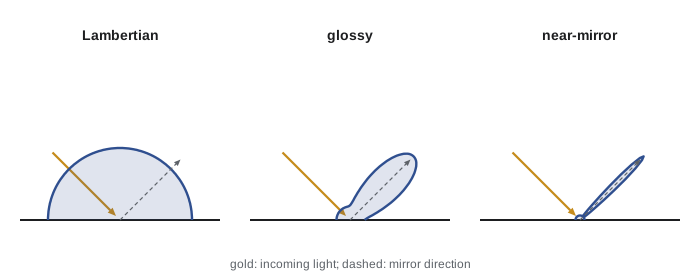
Lambertian diffuse reflection
An ideal diffuse, or Lambertian, surface reflects light equally in all directions, so it looks equally bright from any viewpoint; chalk, matte paint and unfinished wood approximate it. Its BRDF is a constant, \(f_r = \rho/\pi\), where \(\rho\), the albedo, is the fraction of incident light reflected (between 0 and 1, per color channel), and the division by \(\pi\) ensures energy conservation, because integrating \(\cos\theta\) over the hemisphere gives \(\pi\). The reflected radiance from a light of irradiance E at normal incidence is \(L_o = (\rho/\pi)\,E\,\max(n \cdot l, 0)\). The clamp at zero handles surfaces facing away from the light. Real materials are rarely perfectly Lambertian; Oren and Nayar's 1994 model adds roughness-dependent retroreflection for surfaces such as clay and the Moon, which looks flatter than a Lambertian sphere.
Phong and Blinn–Phong
Bui Tuong Phong's 1975 thesis introduced both the interpolation of normals across triangles (Phong shading, as opposed to Gouraud's interpolation of colors) and an empirical reflection model with three terms. The ambient term is a constant standing in for indirect light. The diffuse term is Lambertian. The specular term models shiny highlights as \(k_s (r \cdot v)^s\), where \(r\) is the light direction reflected about the normal, \(v\) points to the viewer and the exponent s controls the size of the highlight: large for polished plastic, small for rough surfaces. James Blinn's 1977 modification uses the half vector \(h = (l + v)/\lVert l + v\rVert\), halfway between the light and view directions, and computes \((n \cdot h)^{s}\). Blinn–Phong is cheaper when the light and viewer are distant, behaves better at grazing angles and, as Blinn noted, corresponds loosely to a distribution of microscopic facets oriented around the normal, which anticipates the physically based models below.
# Lambert diffuse plus Blinn-Phong specular on a sphere, printed as ASCII
# shades, and the individual terms at a few points.
import numpy as np
L = np.array([-0.5, 0.6, 0.62]); L /= np.linalg.norm(L)     # toward the light
V = np.array([0.0, 0.0, 1.0])                                # toward the viewer
H = (L + V) / np.linalg.norm(L + V)                          # half vector
ka, kd, ks, shininess = 0.08, 0.75, 0.5, 40
def shade(n):
    diff = max(n @ L, 0.0)
    spec = max(n @ H, 0.0) ** shininess if diff > 0 else 0.0
    return ka + kd * diff + ks * spec, diff, spec
ramp = " .,:;i1tfLCG08@"
for row in range(11):
    y = 1 - (row + 0.5) / 5.5
    line = ""
    for col in range(32):
        x = (col + 0.5) / 16 - 1
        if x * x + y * y >= 1: line += " "; continue
        n = np.array([x, y, np.sqrt(1 - x * x - y * y)])
        c = min(shade(n)[0], 1.0)
        line += ramp[int(c * (len(ramp) - 1))]
    print(line)
for name, n in (("facing viewer", V), ("toward light", L), ("highlight (n = h)", H), ("away from light", np.array([1.0, 0, 0]))):
    tot, d, s = shade(n)
print(f"{name:18} diffuse {d:.3f} specular {s:.3f} total {tot:.3f}") LCCCCCLLLfft1i
CGGGGGGGCCCCLLfftt1i;:
CGGGG008880GCCLLfftt11i;:,
LCCGGG08@@@@@8GCLfftt11i;;:,..
fLCCCCCG08@@80GLLftt11ii;;:,,...
tfLLLLLLLLLLLffttt11ii;;::,.....
1tttfffffttttt111iii;;::,.......
ii111111111iiii;;:::,,........
:;;;;;;;;;:::,,,..........
..,,,,,...............
..............
facing viewer diffuse 0.622 specular 0.015 total 0.554
toward light diffuse 1.000 specular 0.015 total 0.838
highlight (n = h) diffuse 0.900 specular 1.000 total 1.255
away from light diffuse 0.000 specular 0.000 total 0.080The ASCII sphere shows the classic look: brightness falls off away from the light toward the terminator, where \(n \cdot l = 0\), with a tight highlight where the normal is close to the half vector, and only the ambient term on the side away from the light. The printed terms confirm that the specular term peaks at exactly 1 when n equals h, while a normal facing away from the light receives only the ambient term. The model is cheap and served games for two decades, but it is not energy conserving (a higher exponent makes the highlight smaller without making it brighter), its parameters do not correspond to measurable properties, and materials tuned under one lighting setup look wrong under another.
Interpolation: flat, Gouraud and Phong shading
The lighting model can be evaluated at different places. Flat shading evaluates it once per triangle with the face normal, giving a faceted look. Gouraud shading (1971) evaluates it at the vertices and interpolates the resulting colors across the triangle, which is cheap but misses highlights that fall between vertices and makes them flicker as objects move. Phong shading interpolates normals and evaluates lighting per pixel, which is the norm today in fragment shaders. 'Phong' therefore names both an interpolation method and a reflection model, which causes confusion.
Physically based rendering
Physically based rendering (PBR) builds shading on measurable material properties and on energy conservation, so materials look right under any lighting. Its core is microfacet theory, from Kenneth Torrance and Ephraim Sparrow's 1967 optics work and Robert Cook and Torrance's 1982 graphics paper: a rough surface is modeled as countless tiny mirror facets with a statistical distribution of orientations. Light reflects specularly toward the viewer only from facets whose normal equals the half vector h. The specular BRDF is
D is the normal distribution function, the density of facets oriented along h; the GGX or Trowbridge–Reitz distribution, popularized by Bruce Walter and colleagues in 2007, has a bright core and long tails that match measured materials well. G is the geometric masking-shadowing term, the fraction of those facets visible to both the light and the viewer, usually Smith's form. F is the Fresnel reflectance: the fraction of light reflected rather than refracted at each facet, which rises toward 1 at grazing angles. Christophe Schlick's 1994 approximation \(F \approx F_0 + (1 - F_0)(1 - v \cdot h)^5\) is used almost universally, with \(F_0\), the reflectance at normal incidence, about 0.04 for most dielectrics (plastic, glass, water, skin) and 0.5 to 1.0, colored, for metals.
Brent Burley's 2012 Disney principled BRDF and Brian Karis's 2013 adaptation for Unreal Engine 4 established the parameterization most tools now share, the metallic-roughness workflow. An artist sets a base color, a metallic value (0 for dielectrics, whose base color is the diffuse albedo and whose specular is the gray 0.04; 1 for metals, which have no diffuse reflection and whose base color tints the specular) and a perceptual roughness, typically remapped as \(\alpha = \text{roughness}^2\) for the GGX distribution. This model is standardized in glTF 2.0's materials and in OpenPBR, a material model published through the Academy Software Foundation in 2024 that merges Autodesk's Standard Surface and Adobe's Standard Material.
# A microfacet (Cook-Torrance) specular BRDF with the GGX distribution, Smith
# masking-shadowing and Schlick's Fresnel approximation. We print the peak value
# and the directional albedo (the fraction of light reflected), estimated by
# numerical integration over the hemisphere.
import numpy as np
def D_ggx(nh, a):  return a * a / (np.pi * ((nh * nh) * (a * a - 1) + 1) ** 2)
def G1(nx, a):     return 2 * nx / (nx + np.sqrt(a * a + (1 - a * a) * nx * nx))
def F_schlick(vh, f0): return f0 + (1 - f0) * (1 - vh) ** 5
def brdf(l, v, a, f0):                    # n = (0, 0, 1)
    h = (l + v) / np.linalg.norm(l + v, axis=-1, keepdims=True)
    nl, nv, nh = l[..., 2], v[2], h[..., 2]
    vh = np.clip((v * h).sum(-1), 0, 1)
    return D_ggx(nh, a) * G1(nl, a) * G1(nv, a) * F_schlick(vh, f0) / (4 * nl * nv)
def albedo(v, a, f0, n=400):              # integral of f cos(theta_l) over the hemisphere
    th = (np.arange(n) + 0.5) / n * np.pi / 2
    ph = (np.arange(2 * n) + 0.5) / (2 * n) * 2 * np.pi
    T, P = np.meshgrid(th, ph, indexing="ij")
    l = np.stack([np.sin(T) * np.cos(P), np.sin(T) * np.sin(P), np.cos(T)], -1)
    f = brdf(l, v, a, f0)
    dA = (np.pi / 2 / n) * (2 * np.pi / (2 * n))
    return float((f * np.cos(T) * np.sin(T)).sum() * dA)
v = np.array([np.sin(np.radians(30)), 0, np.cos(np.radians(30))])   # viewer 30 deg off normal
mirror = np.array([-v[0], 0, v[2]])
print("roughness  peak BRDF (mirror dir)  albedo F0=1 (metal-like)  albedo F0=0.04 (dielectric)")
for r in (0.1, 0.3, 0.6, 0.9):
    a = r * r                                            # common remapping alpha = roughness^2
    print(f"{r:9}  {float(brdf(mirror[None], v, a, 1.0)[0]):18.2f}  {albedo(v, a, 1.0):22.3f}  {albedo(v, a, 0.04):24.3f}")
print("Schlick Fresnel for glass (F0 = 0.04) at 0, 60, 80, 89 degrees:",
[round(float(F_schlick(np.cos(np.radians(t)), 0.04)), 3) for t in (0, 60, 80, 89)])roughness peak BRDF (mirror dir) albedo F0=1 (metal-like) albedo F0=0.04 (dielectric)
0.1 1061.02 1.000 0.040
0.3 13.08 0.989 0.040
0.6 0.80 0.811 0.033
0.9 0.15 0.437 0.018
Schlick Fresnel for glass (F0 = 0.04) at 0, 60, 80, 89 degrees: [0.04, 0.07, 0.41, 0.919]As roughness increases, the peak of the specular lobe falls by orders of magnitude while its width grows, so the highlight spreads and dims, unlike Blinn–Phong's. The directional albedo, the fraction of incoming light reflected, stays below 1, so the model does not create energy; for rough metal it falls noticeably below 1, because single-scattering microfacet models ignore light that bounces between facets, which makes rough metals look too dark. Production renderers add a multiple-scattering compensation term to restore that energy. For a dielectric with \(F_0 = 0.04\), only a few percent of light reflects specularly at moderate angles, but Schlick's Fresnel shows reflectance climbing steeply toward grazing incidence, which is why a lake mirrors distant mountains while you can see into the water at your feet.
| Material | Metallic | \(F_0\) (linear) | Notes |
|---|---|---|---|
| Water, glass, plastic | 0 | 0.02 to 0.05 | Gray specular; color comes from diffuse or transmission |
| Skin | 0 | about 0.028 | Needs subsurface scattering for realism |
| Iron | 1 | about (0.56, 0.57, 0.58) | No diffuse; specular is the color |
| Copper | 1 | about (0.95, 0.64, 0.54) | Reddish specular tint |
| Gold | 1 | about (1.00, 0.71, 0.29) | Yellow specular tint |
| Silver | 1 | about (0.95, 0.93, 0.88) | Highest reflectance of common metals |
Light sources
Directional lights model distant sources such as the sun, with a single direction and no falloff. Point lights emit from a position in all directions with inverse-square falloff; spotlights restrict a point light to a cone with a smooth edge. Real lights have area, which produces soft shadows and broad highlights; area lights such as spheres, rectangles and tubes are standard in offline rendering and approximated in real time with techniques such as linearly transformed cosines (2016). Image-based lighting uses a high dynamic range environment map, a photograph of all directions around a point, as a light source surrounding the scene; prefiltering the map for each roughness level lets a single texture lookup approximate the integral of the BRDF over the environment, the split-sum approximation that Karis described in 2013. Lights in physically based engines are specified in photometric units, lumens for bulbs and lux for the sun, so that exposure works like a real camera.
Shadows
A point is in shadow when the path to the light is blocked. Shadows anchor objects to the ground, reveal shape and convey the position of lights, and their absence is one of the most obvious flaws in a rendering. Lance Williams's 1978 shadow mapping is the dominant real-time technique: render the scene's depth from the light's point of view into a texture, the shadow map; then, when shading a point, transform it into the light's view and compare its depth with the stored depth. If the point is farther than the stored value, something nearer to the light blocks it. Shadow maps work with any geometry the rasterizer can draw, but they suffer from sampling problems: aliasing where shadow-map texels are magnified on screen, and shadow acne, false self-shadowing caused by the limited resolution and depth precision of the map.
# Shadow-map acne and bias in one dimension. A light looks straight down on a
# gently sloping floor; the shadow map stores depth per texel, and the floor is
# compared against the stored depth when shading.
import numpy as np
texels = 16                                   # shadow-map resolution across 8 m
xs = (np.arange(64) + 0.5) / 64 * 8           # shading points on the floor
floor = lambda x: 0.35 * x                     # floor height rises 0.35 m per m
store = floor((np.floor(xs / 8 * texels) + 0.5) / texels * 8)   # depth at texel middle
light_h = 10.0
def lit(bias):
    d_point = light_h - floor(xs)             # distance from light to the point
    d_map = light_h - store                    # distance stored in the shadow map
    return d_point <= d_map + bias
for bias in (0.0, 0.05, 0.1, 0.2):
    l = lit(bias)
    print(f"bias {bias:4}: {''.join('#' if s else '.' for s in l)}  lit {l.mean():.0%}")
print("('.' = wrongly shadowed point; the floor is fully lit, so any '.' is acne)")bias 0.0: ..##..##..##..##..##..##..##..##..##..##..##..##..##..##..##..## lit 50%
bias 0.05: .###.###.###.###.###.###.###.###.###.###.###.###.###.###.###.### lit 75%
bias 0.1: ################################################################ lit 100%
bias 0.2: ################################################################ lit 100%
('.' = wrongly shadowed point; the floor is fully lit, so any '.' is acne)With no bias, half of the floor shadows itself in a regular pattern, because within each shadow-map texel the floor rises above the single stored depth; this is acne. A small bias removes it. An excessive bias makes shadows detach from the objects that cast them, an artifact called peter-panning, though the flat floor here cannot show it. Practical renderers use a slope-scaled bias, larger where the surface is steep relative to the light, and normal offsets. Cascaded shadow maps split the view frustum into ranges with separate maps to give more resolution near the camera. Percentage-closer filtering (PCF) averages several shadow comparisons to soften edges, and percentage-closer soft shadows (PCSS) vary the filter width with the distance between blocker and receiver to imitate the penumbra of area lights. Shadow volumes, which extrude silhouette edges into geometry and count crossings in the stencil buffer, give exact hard shadows and were used in games such as Doom 3 (2004), but scale poorly. Ray-traced shadows (lesson 11) are now practical on hardware with ray tracing support.
Ambient occlusion
The constant ambient term of the Phong model makes creases and contact points look flat. Ambient occlusion (AO) scales ambient light by the fraction of the hemisphere above a point that is unoccluded by nearby geometry, darkening corners, cracks and the area under objects. It was introduced in film production by Industrial Light and Magic around 2002 and brought to games by Crytek's screen-space ambient occlusion (SSAO) in Crysis (2007), which estimates occlusion from the depth buffer. Variants such as horizon-based AO and ground-truth AO improve accuracy, and ray-traced AO samples actual geometry. AO is a crude stand-in for global illumination, but it adds a great deal of perceived realism for little cost.
Worked examples
Worked problem
Diffuse irradiance
Sunlight delivers 1,000 W/m² to a surface facing it. What irradiance does a roof tilted 60 degrees from the sun direction receive, and what radiance does a Lambertian roof of albedo 0.3 reflect?
Show solution
- Irradiance: \(1000 \cos 60° = 500\) W/m².
- Radiance: \((0.3/\pi) \times 500 = 47.7\) W/(m²·sr), the same from every viewing direction.
Answer: 500 W/m² of irradiance and about 47.7 W/(m²·sr) of reflected radiance.
Worked problem
Blinn–Phong highlight
With l = (0, 0.6, 0.8) and v = (0, 0, 1), compute the half vector and the specular term for a normal n = (0, 0.316, 0.949) with exponent 50.
Show solution
- \(l + v = (0, 0.6, 1.8)\), length 1.897, so \(h = (0, 0.316, 0.949)\).
- \(n \cdot h = 1.0\), so the specular term is \(1^{50} = 1\): this normal sits exactly at the highlight.
- Tilting n by 5 degrees gives \(n \cdot h = \cos 5° = 0.9962\), and \(0.9962^{50} = 0.83\).
Answer: h = (0, 0.316, 0.949); the highlight term is 1 at this normal and 0.83 five degrees away.
Worked problem
Fresnel at grazing angles
Using Schlick's approximation with F0 = 0.02 for water, compare reflectance looking straight down and at 85 degrees from the normal.
Show solution
- Straight down: \(F = 0.02\).
- At 85 degrees, \(\cos 85° = 0.0872\), \((1 - 0.0872)^5 = 0.634\), so \(F = 0.02 + 0.98 \times 0.634 = 0.641\).
Answer: About 2 percent at normal incidence and 64 percent at 85 degrees: water becomes a mirror at grazing angles.
Common mistakes
MistakeForget the cosine factor n · l, or let it go negative.
InsteadMultiply by max(n · l, 0) for every light.
MistakeUse albedo directly as the Lambertian BRDF.
InsteadThe Lambertian BRDF is \(\rho/\pi\); the \(\pi\) keeps energy conserved.
MistakeGive dielectrics colored specular reflection.
InsteadDielectrics have gray specular near 0.04; colored specular and no diffuse indicate a metal.
MistakeTune materials under one light and assume they will hold up.
InsteadUse physically based, energy-conserving models with measured parameters.
MistakeRemove shadow acne with a large constant bias.
InsteadUse slope-scaled bias and normal offsets; large constant bias causes peter-panning.
Summary and key terms
- Radiance, power per area per solid angle, is what cameras measure and is constant along rays in empty space.
- Lambert's cosine law makes received light proportional to n · l.
- The BRDF describes how a material reflects light; plausible BRDFs are positive, reciprocal and energy conserving.
- Lambertian diffuse has BRDF \(\rho/\pi\); Blinn–Phong adds an empirical highlight \((n \cdot h)^{s}\).
- Microfacet BRDFs combine a normal distribution (GGX), masking-shadowing (Smith) and Fresnel (Schlick).
- The metallic-roughness workflow parameterizes PBR materials in glTF, game engines and OpenPBR.
- Shadow maps, filtering and ambient occlusion supply the shadowing that anchors objects in a scene.
- Radiance
- Power per unit projected area per unit solid angle; the quantity a sensor measures.
- Irradiance
- Power arriving per unit area of a surface.
- BRDF
- Bidirectional reflectance distribution function: reflected radiance per unit incident irradiance.
- Albedo
- The fraction of incident light a surface reflects diffusely.
- Half vector
- The unit vector halfway between the light and view directions.
- Microfacet model
- A reflection model treating a rough surface as many tiny mirror facets.
- Fresnel reflectance
- The fraction of light reflected at an interface, rising toward 1 at grazing angles.
- Metallic-roughness workflow
- A PBR parameterization using base color, metallic and roughness values.
- Shadow map
- A depth image rendered from a light, used to test whether points are shadowed.
- Ambient occlusion
- An estimate of how much of the hemisphere above a point is blocked by nearby geometry.
Practice problems
Work each problem on paper first, then reveal the answer to check.
How many steradians are in a hemisphere?
Show answer
\(2\pi\).
Why does the Lambertian BRDF include a factor of 1/π?
Show answer
Integrating \(\cos\theta\) over the hemisphere gives \(\pi\), so this keeps reflected energy at most the incident energy.
What is the half vector for light and view directions that coincide?
Show answer
The same direction.
What does a larger Blinn–Phong exponent do?
Show answer
Makes the highlight smaller and sharper.
Name the three factors in the numerator of the Cook–Torrance BRDF.
Show answer
D (normal distribution), G (masking-shadowing) and F (Fresnel).
What is a typical F0 for dielectrics?
Show answer
About 0.04.
Why do rough metals look too dark with single-scattering microfacet models?
Show answer
They ignore light that bounces between microfacets before leaving.
What causes shadow acne?
Show answer
Limited shadow-map resolution and depth precision making surfaces shadow themselves.
What is peter-panning?
Show answer
Shadows detaching from their casters because of excessive bias.
What does screen-space ambient occlusion use as input?
Show answer
The depth buffer (and often normals).
Lesson quiz · 5 questions
Score 60% or more to complete this lesson.
Create a free account to save your progress, take quizzes and earn a certificate.