Capstone: global illumination, path tracing and modern rendering

Every technique so far has approximated how light behaves. This final lesson describes the physics the approximations aim at, the rendering equation, and the Monte Carlo method that solves it, path tracing, which is how nearly every animated feature film and much architectural and product visualization is rendered today. It then surveys how real-time graphics is converging on the same ideas through hybrid ray tracing, denoising and neural upscaling; the rise of neural scene representations such as neural radiance fields and Gaussian splatting; the social questions graphics raises, from photosensitive seizures to synthetic media; the industry in Canada and the United States; and a capstone project that brings the course together.

The rendering equation

In 1986 James Kajiya published 'The rendering equation', which unified the field: almost every rendering algorithm can be seen as an approximate solution of one integral equation. The radiance leaving a point x in direction \(\omega_o\) equals the radiance it emits plus the radiance it reflects, gathered from every incoming direction over the hemisphere and weighted by the BRDF (lesson 8) and the cosine factor.

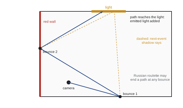
The equation is recursive: the incoming radiance \(L_i\) at x is the outgoing radiance from whatever surface a ray from x in direction \(\omega_i\) hits first, which itself satisfies the same equation. Light therefore bounces indefinitely, and the solution includes direct lighting, indirect lighting (color bleeding from a red wall onto a white floor), soft shadows from area lights, glossy reflections and caustics, the bright patterns focused by glass or water. Methods that account for this interreflection are called global illumination. Whitted ray tracing (lesson 11) solves only the special case of point lights and perfect mirrors; rasterization with local shading solves only the first term of the bounce series.

The earliest practical global illumination method was radiosity, adapted from heat-transfer engineering by Cindy Goral, Donald Greenberg and colleagues at Cornell in 1984. It divides diffuse surfaces into patches, computes form factors describing how much each patch sees of every other, and solves a linear system for the light leaving each patch. Radiosity handles only diffuse surfaces and scales poorly, but its view-independent results could be baked into lightmaps, and baked lighting remains common in games, now computed by GPU path tracers in level editors.

Monte Carlo integration

The rendering equation's integral has no closed form for real scenes, and it is high-dimensional, because each bounce adds two dimensions. Monte Carlo integration estimates an integral \(\int f(x)\,dx\) by drawing random samples \(x_k\) from a probability density p and averaging \(f(x_k)/p(x_k)\). The estimate is unbiased (its expected value is the exact integral) whatever the dimension, and its error falls as \(1/\sqrt{N}\) for N samples. That rate is slow, so quadrupling the samples only halves the noise, but it does not degrade with dimension, which is why Monte Carlo dominates rendering.

The variance, visible as noise, depends on how well p matches the shape of f. Importance sampling chooses p to put samples where f is large. For diffuse surfaces, sampling directions with density proportional to \(\cos\theta\) cancels the cosine factor exactly; for glossy surfaces, sampling the BRDF lobe concentrates samples near the reflection direction; for small bright lights, sampling the light directly (next-event estimation) is essential. Eric Veach's 1997 thesis introduced multiple importance sampling, which combines several sampling strategies with weights so that each handles the cases it is good at, and remains the backbone of production renderers.

# Monte Carlo estimation of the irradiance at a point under a uniform sky of
# radiance 1 (exact answer: pi), comparing uniform hemisphere sampling with
# cosine-weighted importance sampling. Same number of samples, many trials.
import numpy as np
rng = np.random.default_rng(411)
def uniform(n):
    u1 = rng.random(n)                     # cos(theta) uniform on [0, 1]
    cos_t = u1
    pdf = 1 / (2 * np.pi)
    return (1.0 * cos_t / pdf).mean()      # L * cos(theta) / pdf
def cosine(n):
    u1 = rng.random(n)
    cos_t = np.sqrt(u1)                    # Malley's method: pdf = cos(theta)/pi
    pdf = cos_t / np.pi
    return (1.0 * cos_t / pdf).mean()
print(f"exact irradiance = pi = {np.pi:.4f}")
for n in (4, 16, 64, 256):
    a = np.array([uniform(n) for _ in range(2000)])
    b = np.array([cosine(n) for _ in range(2000)])
    print(f"{n:4d} samples  uniform: mean {a.mean():.4f} std {a.std():.4f}   cosine-weighted: mean {b.mean():.4f} std {b.std():.4f}")
# a harder case: a small bright window (the 'sun') covering part of the sky
def window(n, sampler):
    u1, u2 = rng.random(n), rng.random(n)
    if sampler == "uniform":
        cos_t = u1; pdf = np.full(n, 1 / (2 * np.pi))
    else:
        cos_t = np.sqrt(u1); pdf = cos_t / np.pi
    phi = 2 * np.pi * u2
    sin_t = np.sqrt(1 - cos_t ** 2)
    d = np.stack([sin_t * np.cos(phi), sin_t * np.sin(phi), cos_t], 1)
    sun = np.array([0.0, np.sin(0.6), np.cos(0.6)])
    L = np.where(d @ sun > np.cos(0.15), 50.0, 0.2)  # bright disc of half-angle 0.15 rad
    return (L * cos_t / pdf).mean()
a = np.array([window(64, "uniform") for _ in range(2000)])
b = np.array([window(64, "cosine") for _ in range(2000)])
print(f"small bright source, 64 samples: uniform std {a.std():.2f}, cosine std {b.std():.2f}"
      f" (means {a.mean():.2f}, {b.mean():.2f})")

exact irradiance = pi = 3.1416
   4 samples  uniform: mean 3.1138 std 0.9123   cosine-weighted: mean 3.1416 std 0.0000
  16 samples  uniform: mean 3.1357 std 0.4407   cosine-weighted: mean 3.1416 std 0.0000
  64 samples  uniform: mean 3.1416 std 0.2273   cosine-weighted: mean 3.1416 std 0.0000
 256 samples  uniform: mean 3.1379 std 0.1117   cosine-weighted: mean 3.1416 std 0.0000
small bright source, 64 samples: uniform std 3.25, cosine std 2.55 (means 3.45, 3.52)

For a uniform sky, cosine-weighted sampling has zero variance: every sample returns exactly \(\pi\), because the sampling density is exactly proportional to the integrand. Uniform sampling is unbiased too (its mean is close to \(\pi\)) but noisy, and its standard deviation halves each time the sample count quadruples, the \(1/\sqrt{N}\) law. With a small bright source, neither strategy matches the integrand, and both are very noisy because few samples happen to hit the sun; this is the case where sampling the light source directly is needed, which is exactly what next-event estimation and multiple importance sampling do.

Path tracing

Kajiya's path tracing solves the rendering equation by Monte Carlo sampling of light paths. For each pixel, trace a camera ray to the first hit; add the emitted light; sample one new direction from the BRDF (or a mixture of strategies), weight the result by \(f_r \cos\theta / p\), and continue from the next hit, building a path of bounces. At each vertex, next-event estimation also sends a shadow ray to a randomly chosen point on a light. Averaging many such paths per pixel converges to the correct image, including every global illumination effect, with no special cases. Paths must end somewhere: Russian roulette terminates each path with some probability after a few bounces and divides the surviving paths' contribution by the survival probability, which keeps the estimate unbiased while spending little effort on paths that carry little light.

# A small Monte Carlo path tracer for a diffuse "furnace" test and a two-wall
# corner, showing how indirect bounces add light and how Russian roulette
# keeps the estimate unbiased while cutting path length.
import numpy as np
rng = np.random.default_rng(7)
# Furnace test: a closed sphere of albedo rho emitting Le everywhere. Every
# surface sees radiance L = Le / (1 - rho) (geometric series of bounces).
def furnace(rho, Le=1.0, rr=True, max_depth=500):
    L, throughput, depth = 0.0, 1.0, 0
    while depth < max_depth:
        L += throughput * Le
        throughput *= rho                      # diffuse bounce, cosine-sampled: weight = albedo
        depth += 1
        if rr and depth > 3:
            p = min(throughput, 0.95)          # survival probability
            if rng.random() > p: break
            throughput /= p                    # compensate so the expectation is unchanged
    return L, depth
for rho in (0.5, 0.8):
    for rr in (False, True):
        runs = [furnace(rho, rr=rr) for _ in range(20000)]
        est = np.mean([r[0] for r in runs]); length = np.mean([r[1] for r in runs])
        print(f"albedo {rho}  roulette {str(rr):5}: estimate {est:.3f} (exact {1 / (1 - rho):.3f}),"
              f" mean path length {length:6.1f}")
# How much of the light at a point comes from each bounce, for albedo 0.7:
rho = 0.7
print("share of radiance by number of bounces (albedo 0.7):",
      [f"{(1 - rho) * rho ** k:.2f}" for k in range(6)], "...")

albedo 0.5  roulette False: estimate 2.000 (exact 2.000), mean path length  500.0
albedo 0.5  roulette True : estimate 1.999 (exact 2.000), mean path length    4.1
albedo 0.8  roulette False: estimate 5.000 (exact 5.000), mean path length  500.0
albedo 0.8  roulette True : estimate 5.010 (exact 5.000), mean path length    6.1
share of radiance by number of bounces (albedo 0.7): ['0.30', '0.21', '0.15', '0.10', '0.07', '0.05'] ...

The furnace test, a closed environment of uniform emission and albedo, has the exact answer \(L_e/(1-\rho)\), the sum of a geometric series of bounces, so it checks a path tracer's energy bookkeeping. With and without Russian roulette, the estimate matches the exact value, but roulette shortens the average path dramatically, and the gain is greatest for bright materials where paths would otherwise run for hundreds of bounces. The bounce shares show why multiple bounces matter: with albedo 0.7 only 30 percent of the light at a point comes from direct emission, and indirect light is far from negligible in bright interiors, which is why rasterized images without global illumination look flat.

Path tracing has variants for hard cases. Bidirectional path tracing (Lafortune and Willems, 1993; Veach and Guibas, 1994) traces subpaths from both the camera and the lights and connects them, which helps when light enters through small openings. Metropolis light transport (Veach and Guibas, 1997) mutates successful paths to explore difficult light. Photon mapping (Henrik Wann Jensen, 1996) traces photons from lights and stores them, rendering caustics efficiently. Volumetric path tracing handles smoke, clouds and skin. Production renderers using these methods include Pixar's RenderMan (which dropped its older REYES architecture in favor of path tracing with version 21 in 2016), Disney's Hyperion, Autodesk Arnold, Weta FX's Manuka, Blender's Cycles and Chaos V-Ray. The book Physically Based Rendering by Matt Pharr, Wenzel Jakob and Greg Humphreys, now in its fourth edition (2023) and free online, documents the field; Pharr, Humphreys and Pat Hanrahan received a 2014 Academy Scientific and Technical Award for the work behind its first edition.

Denoising and real-time path tracing

Converged film frames take hundreds or thousands of samples per pixel and minutes to hours each. Denoising lets renderers stop much earlier: a filter guided by auxiliary buffers such as albedo, normals and depth smooths noise without blurring edges, and since about 2017 neural denoisers trained on pairs of noisy and converged images, such as NVIDIA's OptiX denoiser, Intel's Open Image Denoise (open source) and the denoisers in Disney and Pixar pipelines, have become standard. Real-time renderers go further, reusing samples across frames with temporal accumulation reprojected by motion vectors, and across pixels with spatiotemporal resampling: ReSTIR (Bitterli and colleagues, 2020) resamples light candidates from neighboring pixels and past frames, making scenes with millions of lights tractable at one or two samples per pixel.

# Why denoisers matter: Monte Carlo error falls as 1/sqrt(N). We estimate a
# pixel whose true value is 0.5 with N noisy samples and report the error, then
# apply a simple 5-tap spatial filter across adjacent pixels of a flat region.
import numpy as np
rng = np.random.default_rng(3)
true = 0.5
print("samples  RMS error   error x sqrt(N)")
for n in (1, 4, 16, 64, 256, 1024):
    est = rng.exponential(true, (4000, n)).mean(1)       # skewed, heavy-ish noise like real renders
    rms = np.sqrt(((est - true) ** 2).mean())
    print(f"{n:7d}  {rms:9.4f}   {rms * np.sqrt(n):9.3f}")
img = rng.exponential(true, (64, 64, 4)).mean(2)          # 4 samples per pixel
k = np.zeros_like(img)
for dy, dx in ((0, 0), (1, 0), (-1, 0), (0, 1), (0, -1)):
    k += np.roll(np.roll(img, dy, 0), dx, 1)
k /= 5
print(f"4 spp image RMS error {np.sqrt(((img - true) ** 2).mean()):.4f};"
      f" after 5-tap filter {np.sqrt(((k - true) ** 2).mean()):.4f}"
      f" (like about {4 * 5} spp, but edges would blur without guidance)")

samples  RMS error   error x sqrt(N)
      1     0.4906       0.491
      4     0.2442       0.488
     16     0.1252       0.501
     64     0.0633       0.507
    256     0.0314       0.503
   1024     0.0158       0.507
4 spp image RMS error 0.2532; after 5-tap filter 0.1132 (like about 20 spp, but edges would blur without guidance)

The product of error and \(\sqrt{N}\) stays roughly constant, confirming the \(1/\sqrt{N}\) law: going from 4 to 1,024 samples, 256 times the work, cuts the error only 16-fold. Averaging five neighboring pixels cuts the error about as much as five times more samples, at no extra rendering cost, which is why denoising is essential, but on real images it blurs edges and texture unless the filter is guided by geometry buffers or learned. Upscalers attack the same budget problem from another side: NVIDIA's DLSS (2018 onward), AMD's FSR and Intel's XeSS render at a lower internal resolution and reconstruct a sharp full-resolution image from the current and previous frames, using neural networks in DLSS, XeSS and FSR 4 (2025). Frame generation synthesizes intermediate frames; DLSS 4, released in January 2025, can generate several frames per rendered frame. These techniques now account for much of the image quality of current games, and they raise new artifacts such as ghosting and smearing under fast motion.

Neural scene representations

A new family of methods represents scenes not as triangles but as learned functions or point sets optimized from photographs. Neural radiance fields (NeRF; Mildenhall and colleagues, 2020) train a small neural network to map a 3D position and viewing direction to density and color, and render novel views by volume rendering along camera rays, from a few dozen photos with known camera poses. Training originally took hours; Instant NGP (Müller and colleagues, 2022) cut it to seconds with multiresolution hash encodings. 3D Gaussian splatting (Kerbl and colleagues, 2023) represents a scene as millions of anisotropic 3D Gaussians with color and opacity, optimized from photos and rasterized by sorting and alpha-blending them (lesson 1's over operator) at real-time frame rates. Splatting spread quickly into commercial capture apps, virtual production and mapping, and research continues on editing, relighting and compressing splats.

Generative models now produce images, video and 3D assets from text, and graphics research increasingly blends physically based rendering with learned components: neural materials that compress complex BRDFs, neural texture compression, learned denoisers and upscalers, and differentiable rendering, which computes gradients of an image with respect to scene parameters so that geometry, materials and lighting can be recovered from photographs by optimization (Mitsuba 3, released in 2022, is a research renderer built for this). The principles of this course, cameras, transformations, sampling, radiometry and visibility, remain the foundation on which these methods are built and evaluated. (The AI courses cover the generative models themselves.)

Graphics and society

Graphics affects people's health and trust. Flashing images can trigger seizures in people with photosensitive epilepsy: the Pokémon episode broadcast in Japan in December 1997 sent hundreds of viewers, mostly children, to hospital. Guidelines limit flashes to no more than three per second, with stricter limits on saturated red flashes; WCAG 2's success criterion 2.3.1 sets this threshold for web content, and broadcasters and game publishers screen content with tools such as the Harding test. Games increasingly offer accessibility settings for motion blur, camera shake, color-blind palettes (lesson 1's color science), subtitles and reduced flashing, and simulator sickness in virtual reality depends on frame rate, latency and how the virtual camera moves.

Photorealistic synthesis undermines the evidential value of images. Deepfakes and generated photographs are used for fraud, harassment and political disinformation, including non-consensual intimate imagery, which several jurisdictions have criminalized. Responses include provenance standards: the Coalition for Content Provenance and Authenticity (C2PA) specification attaches cryptographically signed 'content credentials' recording how an image was captured and edited, supported by some cameras, editing tools and platforms, alongside invisible watermarks embedded by generative models. Neither is foolproof, since metadata can be stripped and watermarks degraded. Graphics practitioners also face questions about labor and authorship as generative tools enter studios, the energy used by rendering farms and model training, and the representation of people of different skin tones, which depends on accurate subsurface scattering and on the diversity of scanned and training data.

The United States is home to many of the companies that defined computer graphics: GPU makers NVIDIA, AMD and Intel; Pixar, Industrial Light and Magic and Walt Disney Animation Studios, whose research groups introduced many techniques in this course; and large game studios and publishers in the Seattle area, California, Texas and elsewhere. University research at Utah (birthplace of Gouraud and Phong shading, texture mapping and the Utah teapot), Cornell (radiosity), Stanford, Berkeley, Carnegie Mellon and many others continues to feed the industry, and SIGGRAPH, the field's main conference, has met in US cities for most of its history. Games and visual effects are also major employers in Canada, whose provincial tax credits attract many productions that US studios lead, so careers in the field often cross the border.

Capstone project: a small renderer

The capstone asks you to build and evaluate a renderer that combines the course's techniques. A suggested scope is a path tracer, written in a language of your choice (Python with NumPy for clarity, or C++, Rust or a GPU compute shader for speed), that loads a small triangle-mesh scene in OBJ or glTF format; builds a BVH with the surface area heuristic (lesson 11); generates camera rays with jittered antialiasing (lessons 2, 4 and 5); supports Lambertian and GGX microfacet materials with metallic-roughness parameters and textures (lessons 8 and 9); uses cosine-weighted sampling, next-event estimation and Russian roulette; and writes linear radiance to an image with correct sRGB encoding and simple tone mapping (lesson 1). Validate it with the furnace test, a Cornell box comparison against a reference renderer such as Mitsuba or Blender Cycles, and convergence plots showing error against samples per pixel.

A good project report states its rendering equation assumptions, shows images at several sample counts, measures performance (rays per second, BVH build time, traversal steps per ray), discusses at least one limitation honestly (for example caustics through glass, which unidirectional path tracing renders poorly), and documents sources for any assets used under their licenses. An alternative capstone is a real-time rasterizer in WebGPU, Vulkan or OpenGL with shadow mapping, physically based shading, mipmapped textures and a performance budget, as the planning example below illustrates.

# Capstone planning: a frame-time budget for a 60 frame-per-second game at
# 2560 x 1440, and the ray budget for ray-traced effects, using illustrative
# throughput figures (assumptions, not measurements of any product).
fps = 60
frame_ms = 1000 / fps
passes = {"geometry and visibility (raster)": 3.0, "shadows (ray traced, 1 ray/px)": 1.6,
          "reflections (ray traced, 0.5 ray/px)": 1.4, "global illumination (1 ray/px)": 2.4,
          "denoising and temporal accumulation": 1.8, "post-processing and upscaling": 1.5,
          "UI and composition": 0.6}
used = sum(passes.values())
for k, v in passes.items():
    print(f"{k:40} {v:5.1f} ms")
print(f"{'total':40} {used:5.1f} ms of {frame_ms:.1f} ms -> headroom {frame_ms - used:.1f} ms")
w, h = 2560, 1440
internal = (w // 1.5) * (h // 1.5)                 # render at 2/3 resolution, then upscale
rays = internal * (1 + 0.5 + 1)                    # shadow + reflection + GI rays per pixel
assumed_rate = 5e9                                 # rays per second (illustrative)
print(f"internal resolution {int(w // 1.5)} x {int(h // 1.5)}: {rays / 1e6:.1f} M rays per frame,"
      f" {rays * fps / 1e9:.2f} G rays per second needed")
print(f"at an assumed {assumed_rate / 1e9:.0f} G rays/s the rays alone take {1000 * rays / assumed_rate:.2f} ms")

geometry and visibility (raster)           3.0 ms
shadows (ray traced, 1 ray/px)             1.6 ms
reflections (ray traced, 0.5 ray/px)       1.4 ms
global illumination (1 ray/px)             2.4 ms
denoising and temporal accumulation        1.8 ms
post-processing and upscaling              1.5 ms
UI and composition                         0.6 ms
total                                     12.3 ms of 16.7 ms -> headroom 4.4 ms
internal resolution 1706 x 960: 4.1 M rays per frame, 0.25 G rays per second needed
at an assumed 5 G rays/s the rays alone take 0.82 ms

The budget shows why real-time rendering is an exercise in trade-offs. At 60 frames per second, the whole frame must fit in 16.7 milliseconds, so ray-traced effects get roughly one ray per pixel each, at reduced internal resolution, with denoising and upscaling consuming a substantial share. The throughput figure is an assumption for planning, not a measured specification; a real project would profile on target hardware with tools such as RenderDoc, PIX or NVIDIA Nsight and adjust the plan. The same thinking, estimating costs, measuring, and spending effort where it changes the image most, applies to offline rendering, where the budget is hours per frame rather than milliseconds.

Where to go next

Graphics connects to many other fields. Computer vision (see the AI courses) inverts the rendering process to recover scenes from images; robotics (see the robotics courses) uses simulation and rendering to train and test perception; scientific visualization renders volumes and flows; virtual and augmented reality add tracking, stereo and latency constraints; and computational fabrication turns digital geometry into physical objects. The annual SIGGRAPH and SIGGRAPH Asia conferences, the Eurographics Symposium on Rendering, High-Performance Graphics, and open resources such as Physically Based Rendering, Real-Time Rendering (fourth edition, 2018) and the Khronos and W3C specifications are the places to follow the field as it continues to change.

Worked examples