Ray tracing and acceleration structures

Rasterization asks, for each triangle, which pixels it covers. Ray tracing asks the opposite question: for each pixel, which surface does a ray through it hit first? Because it follows the paths light actually takes, ray tracing handles reflections, refractions and shadows naturally, and it is the foundation of physically based offline rendering. For decades it was too slow for real time; since 2018, GPUs with dedicated ray tracing hardware have made it part of games as well. This lesson covers generating rays, intersecting them with geometry, Whitted-style recursive ray tracing with shadows, reflection and refraction, and the acceleration structures, above all bounding volume hierarchies, that make ray tracing millions of triangles practical. Lesson 12 extends it to global illumination with Monte Carlo path tracing.

Rays and ray generation

A ray is a half-line \(r(t) = o + t\,d\) with origin o, direction d (usually normalized) and parameter \(t \ge 0\). Primary or camera rays start at the eye and pass through each pixel of a virtual image plane. With the camera looking down \(-z\), a vertical field of view \(\theta\) and aspect ratio a, the pixel \((i, j)\) of a \(W \times H\) image has normalized device coordinates \(x = (2(i + 0.5)/W - 1)\,a\tan(\theta/2)\) and \(y = (1 - 2(j + 0.5)/H)\tan(\theta/2)\), and the ray direction in camera space is \((x, y, -1)\), normalized and then rotated into world space by the inverse view matrix of lesson 4. Sampling several jittered positions within each pixel and averaging is the ray tracer's form of supersampling antialiasing (lesson 2), and sampling over a lens aperture or over time gives depth of field and motion blur almost for free.

Ray–object intersection

The core operation is finding the smallest positive t at which a ray meets a surface. For an implicit surface \(f(p) = 0\), substitute \(p = o + t\,d\) and solve for t. A sphere with center c and radius r gives the quadratic \(\lVert o + t d - c\rVert^2 = r^2\), that is \(t^2 + 2b\,t + C = 0\) with \(b = (o - c)\cdot d\) and \(C = \lVert o - c\rVert^2 - r^2\) for unit d. A negative discriminant means a miss; otherwise the nearer root is the entry point, unless it is behind the origin, in which case the ray started inside and the far root is the exit. A plane \(n \cdot p = k\) gives \(t = (k - n \cdot o)/(n \cdot d)\), with no hit if \(n \cdot d = 0\).

Triangles matter most, because meshes are made of them. The Möller–Trumbore algorithm (1997) solves \(o + t d = (1 - u - v)v_0 + u v_1 + v v_2\) directly for t and the barycentric coordinates \((u, v)\) using Cramer's rule with cross and dot products, without first computing the triangle's plane. The ray hits if \(u \ge 0\), \(v \ge 0\), \(u + v \le 1\) and \(t > 0\). The barycentric coordinates it returns are exactly what is needed to interpolate normals and texture coordinates at the hit point. Robust implementations, such as the watertight algorithm of Woop, Benthin and Wald (2013), avoid rays slipping through the shared edges of adjacent triangles because of floating-point rounding.

# Ray-sphere and ray-triangle (Moller-Trumbore) intersection, with checks.
import numpy as np
def hit_sphere(o, d, c, r):
    oc = o - c
    b = oc @ d; cc = oc @ oc - r * r            # d is unit length, so a = 1
    disc = b * b - cc
    if disc < 0: return None
    s = np.sqrt(disc)
    for t in (-b - s, -b + s):                   # nearest positive root
        if t > 1e-6: return t
    return None
def hit_triangle(o, d, v0, v1, v2, eps=1e-9):
    e1, e2 = v1 - v0, v2 - v0
    p = np.cross(d, e2); det = e1 @ p
    if abs(det) < eps: return None               # ray parallel to triangle
    inv = 1.0 / det; s = o - v0
    u = (s @ p) * inv
    if u < 0 or u > 1: return None
    q = np.cross(s, e1); v = (d @ q) * inv
    if v < 0 or u + v > 1: return None
    t = (e2 @ q) * inv
    return (t, u, v) if t > 1e-6 else None
o = np.array([0.0, 0.0, 0.0])
d = np.array([0.0, 0.0, -1.0])
print("sphere at z=-5, r=1:", hit_sphere(o, d, np.array([0, 0, -5.0]), 1.0))
print("sphere off to the side:", hit_sphere(o, d, np.array([3, 0, -5.0]), 1.0))
print("ray starting inside sphere:", hit_sphere(np.array([0, 0, -5.0]), d, np.array([0, 0, -5.0]), 1.0))
v0, v1, v2 = np.array([-1, -1, -3.0]), np.array([1, -1, -3.0]), np.array([0, 1, -3.0])
t, u, w = hit_triangle(o, d, v0, v1, v2)
print(f"triangle: t = {t:.3f}, barycentric (1-u-v, u, v) = ({1 - u - w:.3f}, {u:.3f}, {w:.3f})")
print("point from t:", o + t * d, " point from barycentrics:", (1 - u - w) * v0 + u * v1 + w * v2)
print("ray missing triangle:", hit_triangle(np.array([2.0, 0, 0]), d, v0, v1, v2))

sphere at z=-5, r=1: 4.0
sphere off to the side: None
ray starting inside sphere: 1.0
triangle: t = 3.000, barycentric (1-u-v, u, v) = (0.250, 0.250, 0.500)
point from t: [ 0.  0. -3.]  point from barycentrics: [ 0.  0. -3.]
ray missing triangle: None

The ray hits the sphere centered at z = −5 at t = 4, its near surface; the off-axis sphere is missed; a ray starting at the sphere's center exits at t = 1. The triangle is hit at t = 3, and the point reconstructed from the barycentric weights equals the point along the ray, which is the check that the solution is right. The small threshold (1e-6) on t is essential: rays leaving a surface, such as shadow and reflection rays, would otherwise hit the surface they start on because of rounding, causing speckled self-intersection called surface acne.

Whitted ray tracing

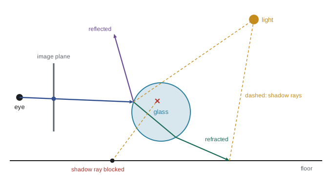
Turner Whitted's 1980 paper 'An improved illumination model for shaded display' defined recursive ray tracing. At the first hit of a camera ray, the renderer computes local shading (lesson 8) and spawns further rays. A shadow ray toward each light determines whether the light is visible; if any object lies between the point and the light, the light contributes nothing. If the surface is a mirror, a reflection ray in the direction \(r = d - 2(d \cdot n)n\) is traced recursively and its result added, weighted by the reflectance. If the surface is transparent, a refraction ray is traced through it in the direction given by Snell's law. Recursion stops at a maximum depth or when the contribution becomes negligible. Whitted's images of glass spheres over a checkerboard became the emblem of the technique.

# A tiny Whitted-style ray tracer: two spheres on a checkered floor, one light,
# hard shadows and one level of mirror reflection, rendered as 60 x 18 ASCII.
import numpy as np
spheres = [(np.array([-1.0, 1.0, -4.0]), 1.0, 0.0),    # middle point, radius, mirror fraction
           (np.array([1.3, 0.8, -3.4]), 0.8, 0.6)]
light = np.array([-4.0, 6.0, 1.0])
def trace_hit(o, d):
    best, hit = np.inf, None
    for c, r, m in spheres:
        oc = o - c; b = oc @ d; disc = b * b - (oc @ oc - r * r)
        if disc > 0:
            t = -b - np.sqrt(disc)
            if 1e-4 < t < best: best, hit = t, ("sphere", c, m)
    if d[1] < -1e-6:
        t = -o[1] / d[1]
        if 1e-4 < t < best: best, hit = t, ("floor", None, 0.0)
    return best, hit
def shade(o, d, depth=0):
    t, hit = trace_hit(o, d)
    if hit is None: return 0.0                        # sky (blank)
    p = o + t * d
    kind, c, mirror = hit
    n = (p - c) / np.linalg.norm(p - c) if kind == "sphere" else np.array([0.0, 1.0, 0.0])
    albedo = 0.8 if kind == "sphere" else (0.75 if (int(np.floor(p[0])) + int(np.floor(p[2]))) % 2 else 0.25)
    to_l = light - p; dist = np.linalg.norm(to_l); l = to_l / dist
    ts, _ = trace_hit(p + 1e-3 * n, l)               # shadow ray
    lit = 0.0 if ts < dist else max(n @ l, 0.0)
    local = 0.05 + albedo * lit
    if mirror > 0 and depth < 2:
        r = d - 2 * (d @ n) * n                       # mirror reflection
        return (1 - mirror) * local + mirror * shade(p + 1e-3 * n, r, depth + 1)
    return local
W, H = 60, 18
ramp = " .:-=+*#%@"
for j in range(H):
    row = ""
    for i in range(W):
        x = (i + 0.5) / W * 2 - 1; y = 1 - (j + 0.5) / H * 2
        d = np.array([x * 1.1, y * 0.42 - 0.12, -1.0]); d /= np.linalg.norm(d)
        v = min(shade(np.array([0.0, 1.2, 1.0]), d), 0.999)
        row += ramp[int(v * len(ramp))]
    print(row)

                                                            
                                                            
                                                            
                      %##*=                                 
                    %%%#**+-.        ::                     
                   ####**+=-.      ---::..                  
                   ##**++=-:.     ----:::.                  
.. . ..:..:.:.:.:..++++==-:.  :.:-+-::::.. .: . . .. . . .  
.---..--..--...--..====--:.   ..-:--:::...  .--:..::..::...:
.===...===....===..:-:::.    =....+-+--=:-....----...---...-
++++::::+++++::::+++ .            :===::.-. ===.....==--....
***:::::******:::::**           +++......       ....=====...
****:::::::******:::::::***+++::::::+         ::.=======....
********:::::::********:::::::**+++++::::::::+++++++:.......
####:::::::::********:::::::::*****++++::::::::+++++++++:::.
:##########:::::::::**********::::::::::+++++++++::::::::::+
#########::::::::::***********:::::::::::++++++++++:::::::::
#######:::::::::::************::::::::::::+++++++++++:::::::

Even at 60 × 18 characters the image shows the essential effects: the checkered floor, two shaded spheres, a hard shadow cast by each sphere onto the floor, and the right-hand sphere reflecting the floor in its lower half because 60 percent of its color comes from the reflection ray. The whole renderer is about forty lines, which is ray tracing's great appeal: effects that need special tricks in a rasterizer (shadow maps, reflection probes, lesson 8 and lesson 9) fall out of one recursive function. What it lacks is everything Whitted's method cannot model: soft shadows from area lights, glossy reflections, diffuse interreflection and caustics, which need the Monte Carlo methods of lesson 12.

Refraction and Fresnel

At a boundary between media with refractive indices \(n_1\) and \(n_2\) (about 1.0 for air, 1.33 for water and 1.5 for glass), the transmitted ray bends according to Snell's law, \(n_1 \sin\theta_1 = n_2 \sin\theta_2\). In vector form, with unit incident direction d and normal n facing the incoming side, \(t = \eta d + (\eta c_1 - c_2)n\), where \(\eta = n_1/n_2\), \(c_1 = -n \cdot d\) and \(c_2 = \sqrt{1 - \eta^2(1 - c_1^2)}\). When light passes into a less dense medium beyond the critical angle \(\arcsin(n_2/n_1)\), the square root becomes imaginary and all light is reflected: total internal reflection, which makes diamonds sparkle and optical fibers work. The split between reflected and refracted light is given by the Fresnel equations, of which Schlick's approximation (lesson 8) is the usual shortcut.

# Refraction with Snell's law and the exact (unpolarized) Fresnel reflectance
# for light going from air into glass (n = 1.5) and from glass into air.
import math
def fresnel(cos_i, n1, n2):
    sin_t = n1 / n2 * math.sqrt(max(0.0, 1 - cos_i ** 2))
    if sin_t >= 1: return 1.0, None                       # total internal reflection
    cos_t = math.sqrt(1 - sin_t ** 2)
    rs = ((n1 * cos_i - n2 * cos_t) / (n1 * cos_i + n2 * cos_t)) ** 2
    rp = ((n1 * cos_t - n2 * cos_i) / (n1 * cos_t + n2 * cos_i)) ** 2
    return (rs + rp) / 2, math.degrees(math.asin(sin_t))
print("angle   air->glass: R   refracted     glass->air: R   refracted")
for deg in (0, 30, 41, 42, 60, 80):
    c = math.cos(math.radians(deg))
    r1, t1 = fresnel(c, 1.0, 1.5); r2, t2 = fresnel(c, 1.5, 1.0)
    s1 = f"{t1:6.1f} deg" if t1 is not None else "   TIR   "
    s2 = f"{t2:6.1f} deg" if t2 is not None else "   total internal reflection"
    print(f"{deg:4d}    {r1:13.3f}   {s1}   {r2:13.3f}   {s2}")
print(f"critical angle glass->air: {math.degrees(math.asin(1 / 1.5)):.1f} deg")

angle   air->glass: R   refracted     glass->air: R   refracted
   0            0.040      0.0 deg           0.040      0.0 deg
  30            0.042     19.5 deg           0.055     48.6 deg
  41            0.046     25.9 deg           0.380     79.8 deg
  42            0.047     26.5 deg           1.000      total internal reflection
  60            0.089     35.3 deg           1.000      total internal reflection
  80            0.388     41.0 deg           1.000      total internal reflection
critical angle glass->air: 41.8 deg

Entering glass, reflectance is 4 percent at normal incidence and rises only slowly until grazing angles. Leaving glass, the ray bends away from the normal, and beyond the critical angle of 41.8 degrees all light is reflected. A ray tracer handles this by checking whether the ray is entering or leaving (the sign of \(n \cdot d\)), flipping the normal and swapping the indices accordingly, and tracing only a reflection ray when the refraction direction does not exist. Colored glass also absorbs light along its path according to Beer's law, so thicker parts look darker, and dispersion, the variation of refractive index with wavelength, splits white light into rainbows when the renderer traces several wavelengths.

The cost of ray tracing and acceleration structures

A naive ray tracer tests every ray against every primitive. A 1920 × 1080 image has about two million pixels; with several rays per pixel and scenes of millions of triangles, brute force needs on the order of \(10^{13}\) intersection tests per frame. Acceleration structures organize primitives spatially so that each ray tests only a few, reducing the cost per ray from linear to roughly logarithmic in the number of primitives. Two families exist. Spatial subdivisions divide space into cells: uniform grids, octrees, and kd-trees, which split space with axis-aligned planes and were the fastest structure for static scenes in the 2000s. Object hierarchies group primitives: bounding volume hierarchies (BVHs) wrap groups of objects in simple bounding volumes, almost always axis-aligned bounding boxes (AABBs), nested in a tree. BVHs now dominate, because they bound memory use, update easily when objects move and map well to hardware.

Testing a ray against an AABB uses the slab method of Kay and Kajiya (1986): compute the t values at which the ray enters and leaves the pair of planes bounding each axis, take the largest entry and the smallest exit, and report a hit if entry is no later than exit. It needs only a few multiplications with precomputed reciprocal direction components. Traversal starts at the root; if the ray misses a node's box, the whole subtree is skipped; otherwise the children are visited, nearer child first, and any subtree whose box is entered only beyond the nearest hit found so far is pruned.

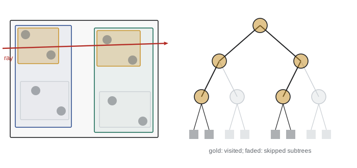
How a BVH is built determines how fast it is. The surface area heuristic (SAH), formulated by Goldsmith and Salmon in 1987 and MacDonald and Booth in 1990, estimates the cost of a split: the probability that a random ray hitting a parent box also hits a child box is the ratio of their surface areas, so a good split minimizes \(\sum_{\text{children}} A_{\text{child}} N_{\text{child}} / A_{\text{parent}}\), weighted by the costs of traversal and intersection. Builders evaluate candidate splits along each axis, often in bins rather than at every primitive, to make construction fast. Real-time engines build a two-level structure: a bottom-level acceleration structure (BLAS) per mesh and a top-level structure (TLAS) over instances of those meshes, rebuilt or refitted every frame as objects move.

# Building a bounding volume hierarchy over random boxes with the surface area
# heuristic (SAH, binned) and counting the work to find the nearest hit for
# random rays, compared with testing every box.
import numpy as np
rng = np.random.default_rng(411)
N = 2000
mids = rng.uniform(0, 100, (N, 3)); half = rng.uniform(0.2, 1.0, (N, 3))
lo_all, hi_all = mids - half, mids + half
def area(lo, hi):
    e = hi - lo; return 2 * (e[0] * e[1] + e[1] * e[2] + e[2] * e[0])
def build(idx, depth=0):
    lo, hi = lo_all[idx].min(0), hi_all[idx].max(0)
    if len(idx) <= 4: return ("leaf", lo, hi, idx)
    best = (np.inf, None, None)
    c = mids[idx]
    for axis in range(3):                          # 12 bins per axis
        cmin, cmax = c[:, axis].min(), c[:, axis].max()
        if cmax - cmin < 1e-9: continue
        for k in range(1, 12):
            split = cmin + (cmax - cmin) * k / 12
            L = idx[c[:, axis] < split]; R = idx[c[:, axis] >= split]
            if len(L) == 0 or len(R) == 0: continue
            cost = (area(lo_all[L].min(0), hi_all[L].max(0)) * len(L) +
                    area(lo_all[R].min(0), hi_all[R].max(0)) * len(R))
            if cost < best[0]: best = (cost, L, R)
    if best[1] is None: return ("leaf", lo, hi, idx)
    return ("node", lo, hi, build(best[1], depth + 1), build(best[2], depth + 1))
def slab(o, inv, lo, hi):
    t1 = (lo - o) * inv; t2 = (hi - o) * inv
    tmin = np.minimum(t1, t2).max(); tmax = np.maximum(t1, t2).min()
    return tmin if tmax >= max(tmin, 0) else np.inf
def nearest(node, o, inv, best, counts):
    counts[0] += 1
    if slab(o, inv, node[1], node[2]) >= best: return best
    if node[0] == "leaf":
        for i in node[3]:
            counts[1] += 1
            best = min(best, slab(o, inv, lo_all[i], hi_all[i]))
        return best
    a, b = node[3], node[4]                         # visit the nearer child first
    if slab(o, inv, b[1], b[2]) < slab(o, inv, a[1], a[2]): a, b = b, a
    best = nearest(a, o, inv, best, counts)
    return nearest(b, o, inv, best, counts)
root = build(np.arange(N))
tests, agree = [], 0
for _ in range(200):
    o = rng.uniform(0, 100, 3); d = rng.normal(size=3); d /= np.linalg.norm(d)
    inv = 1.0 / np.where(np.abs(d) < 1e-12, 1e-12, d)
    counts = [0, 0]
    t_bvh = nearest(root, o, inv, np.inf, counts)
    t_all = min(slab(o, inv, lo_all[i], hi_all[i]) for i in range(N))
    agree += (t_bvh == t_all); tests.append(counts[0] + counts[1])
print(f"{N} boxes, 200 random rays")
print(f"brute force: {N} box tests per ray")
print(f"BVH: mean {np.mean(tests):.0f} node+box tests per ray (median {np.median(tests):.0f}),"
      f" speed-up about {N / np.mean(tests):.0f}x")
print(f"nearest hit identical to brute force for {agree} of 200 rays")

2000 boxes, 200 random rays
brute force: 2000 box tests per ray
BVH: mean 42 node+box tests per ray (median 34), speed-up about 48x
nearest hit identical to brute force for 200 of 200 rays

For 2,000 boxes, the BVH finds the same nearest hit as brute force for every ray while performing only a small fraction of the tests, and the advantage grows with scene size because the tree depth grows only logarithmically. Real scenes are more favorable still, because their geometry is clustered. The Python here is slow in absolute terms; production ray tracers such as Intel's Embree on CPUs and the hardware units of GPUs process hundreds of millions to billions of rays per second using wide trees (four or eight children per node), compressed nodes, and SIMD tests of many boxes or rays at once.

Ray tracing hardware and APIs

Ray tracing entered real-time graphics in 2018. Microsoft added DirectX Raytracing (DXR) to Direct3D 12, NVIDIA launched its Turing GPUs with RT cores that perform BVH traversal and ray–triangle tests in fixed-function hardware, and Battlefield V shipped ray-traced reflections. Vulkan added ray tracing extensions in 2020, Apple added ray tracing to Metal, and AMD's RDNA 2 GPUs (2020), which power the PlayStation 5 and Xbox Series X|S, brought hardware ray tracing to consoles. The programming model adds new shader types: ray generation shaders launch rays, intersection shaders handle custom primitives, any-hit shaders handle transparency such as foliage cut-outs, closest-hit shaders shade the nearest hit, and miss shaders return the sky. Ray queries also let ordinary shaders trace rays inline.

Even with hardware, real-time budgets allow only about one or two rays per pixel per effect, so games use hybrid rendering: rasterize primary visibility, then trace rays for shadows, reflections, ambient occlusion or global illumination, and rely on temporal accumulation and denoising (lesson 12) to clean up the noisy results. Fully path-traced modes, such as Cyberpunk 2077's Overdrive mode (2023) and Alan Wake 2 (2023), show where the technology is heading. On the web, the core WebGPU standard does not include hardware ray tracing as of 2026, though ray tracers written as compute shaders run in browsers.

Beyond triangles

Ray tracing handles any geometry with an intersection routine: exact spheres, NURBS surfaces solved by Newton iteration, subdivision surfaces, curves for hair and fur (ray tracing millions of hair strands is a staple of film renderers), volumes, and implicit surfaces and signed distance fields, which are rendered by sphere tracing (Hart, 1996): step along the ray by the distance-field value, which is guaranteed not to overshoot the surface. Instancing is cheap because a transformed copy of a mesh needs only its transformation, not its own geometry: the ray is transformed into the object's space instead. This lets film scenes contain billions of instanced triangles, such as the forests and crowds of modern visual effects.

Worked examples