Curves, surfaces and animation basics

Triangle meshes are the currency of rendering, but they are not how designers think about smooth shapes or how animators think about motion. The body of a car, the outline of a letter in a font and the path of a camera through a scene are described by smooth parametric curves and surfaces controlled by a handful of points. Motion is described by keyframes interpolated over time, by skeletons that deform meshes, and by physical simulation. This lesson introduces Bézier curves and the de Casteljau algorithm, splines and continuity, the surfaces built from them, and the foundations of computer animation: keyframing and easing, rotations in time, skeletal skinning, inverse kinematics and particle simulation.

Parametric curves

A parametric curve is a function \(p(t)\) from a parameter t, usually in \([0, 1]\), to points in the plane or in space. Unlike an implicit curve \(f(x, y) = 0\), it is easy to draw: evaluate it at a sequence of t values and connect the points. Its derivative \(p'(t)\) is the tangent vector, whose direction gives the curve's direction and whose length gives the speed at which the parameter traces it. Polynomial curves are favored because they are cheap to evaluate and differentiate, and cubics, of degree three, are the lowest degree that can have an inflection point and match a position and tangent at both ends.

Bézier curves and de Casteljau's algorithm

Bézier curves were developed independently in the early 1960s by Paul de Casteljau at Citroën and Pierre Bézier at Renault, both for designing car bodies. A Bézier curve of degree n is defined by n + 1 control points \(P_0, \dots, P_n\). De Casteljau's algorithm evaluates it by repeated linear interpolation: interpolate each consecutive pair of control points at parameter t, giving n points; interpolate those, giving n − 1; and continue until one point remains, which lies on the curve. The same curve can be written with the Bernstein polynomials \(B_{i,n}(t) = \binom{n}{i}(1-t)^{n-i}t^i\) as weights on the control points.

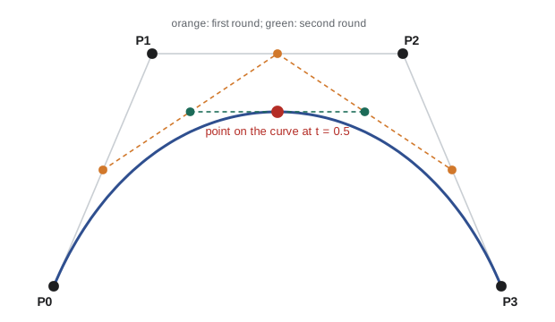
Bézier curves have properties that make them easy to design with. They pass through the first and last control points and are tangent there to the first and last legs of the control polygon; the intermediate control points act as handles that pull the curve without lying on it. The curve lies within the convex hull of its control points, which makes bounding boxes and intersection tests cheap. It is affine invariant: transforming the control points transforms the curve, so there is no need to transform sampled points. And de Casteljau's algorithm subdivides the curve: the intermediate points computed at t = 0.5 are exactly the control points of the two halves, so a renderer can split a curve recursively until each piece is flat enough to draw as a line.

# De Casteljau's algorithm for a cubic Bezier curve, compared with the
# Bernstein-polynomial form, plus subdivision of the curve at t = 0.5.
import numpy as np
P = np.array([[0.0, 0.0], [1.0, 2.0], [3.0, 2.0], [4.0, 0.0]])
def casteljau(P, t):
    pts = [P]
    while len(pts[-1]) > 1:
        Q = pts[-1]
        pts.append((1 - t) * Q[:-1] + t * Q[1:])   # repeated linear interpolation
    return pts
def bernstein(P, t):
    n = len(P) - 1
    from math import comb
    return sum(comb(n, i) * (1 - t) ** (n - i) * t ** i * P[i] for i in range(n + 1))
for t in (0.0, 0.25, 0.5, 0.75, 1.0):
    a = casteljau(P, t)[-1][0]; b = bernstein(P, t)
    print(f"t={t:4.2f}  de Casteljau {a.round(4)}  Bernstein {b.round(4)}")
levels = casteljau(P, 0.5)
left = np.array([lv[0] for lv in levels]); right = np.array([lv[-1] for lv in levels][::-1])
print("left half control points: ", left.round(3).tolist())
print("right half control points:", right.round(3).tolist())
d0 = 3 * (P[1] - P[0]); d1 = 3 * (P[3] - P[2])
print("tangent at start", d0, " tangent at end", d1)

t=0.00  de Casteljau [0. 0.]  Bernstein [0. 0.]
t=0.25  de Casteljau [0.9062 1.125 ]  Bernstein [0.9062 1.125 ]
t=0.50  de Casteljau [2.  1.5]  Bernstein [2.  1.5]
t=0.75  de Casteljau [3.0938 1.125 ]  Bernstein [3.0938 1.125 ]
t=1.00  de Casteljau [4. 0.]  Bernstein [4. 0.]
left half control points:  [[0.0, 0.0], [0.5, 1.0], [1.25, 1.5], [2.0, 1.5]]
right half control points: [[2.0, 1.5], [2.75, 1.5], [3.5, 1.0], [4.0, 0.0]]
tangent at start [3. 6.]  tangent at end [ 3. -6.]

De Casteljau's algorithm and the Bernstein form agree to every printed digit. The left half's control points run from \(P_0\) to the midpoint (2, 1.5), and the right half's from there to \(P_3\); both halves share the midpoint and the tangent there, so the subdivided curve is identical to the original. The end tangents are three times the first and last legs of the control polygon, so moving \(P_1\) changes the starting direction and speed. Bézier curves are everywhere: quadratic Béziers define TrueType font outlines, cubic Béziers define PostScript, PDF, OpenType CFF fonts and SVG paths, and the pen tool in every vector drawing program edits cubic Bézier handles.

Splines and continuity

One Bézier curve of high degree is hard to control: moving any control point changes the whole curve, and high-degree polynomials oscillate. Instead, long curves are built from piecewise cubic segments joined end to end, called splines (after the flexible strips draftsmen bent around weights). How smoothly the pieces join is measured by continuity. \(C^0\) continuity means the segments meet; \(C^1\) means their first derivatives match at the join, so a moving point has no jump in velocity; \(C^2\) means second derivatives match, so there is no jump in acceleration or curvature, which matters for car bodies, where reflections of lights reveal curvature breaks. Geometric continuity \(G^1\) relaxes \(C^1\): the tangent directions must match but their lengths may differ, which looks smooth but changes the parameter speed.

# Joining two cubic Bezier segments: checking C0, C1 and G1 continuity at the
# shared point, then evaluating a uniform cubic B-spline, which is C2 by construction.
import numpy as np
A = np.array([[0, 0], [1, 2], [2, 2], [3, 1]], float)      # first segment
B_c1 = np.array([[3, 1], [4, 0], [5, 1], [6, 2]], float)   # second segment, mirrored handle
B_g1 = np.array([[3, 1], [5, -1], [6, 1], [7, 2]], float)  # same direction, longer handle
def check(A, B):
    c0 = np.allclose(A[3], B[0])
    ta, tb = 3 * (A[3] - A[2]), 3 * (B[1] - B[0])
    c1 = c0 and np.allclose(ta, tb)
    cosang = ta @ tb / (np.linalg.norm(ta) * np.linalg.norm(tb))
    g1 = c0 and abs(cosang - 1) < 1e-9
    return c0, c1, g1, ta, tb
for name, B in (("mirrored handle", B_c1), ("longer handle", B_g1)):
    c0, c1, g1, ta, tb = check(A, B)
    print(f"{name:16} C0={c0} C1={c1} G1={g1}  end tangent {ta} start tangent {tb}")
# uniform cubic B-spline segment basis (Catmull and Clark's surfaces generalize this)
M = np.array([[-1, 3, -3, 1], [3, -6, 3, 0], [-3, 0, 3, 0], [1, 4, 1, 0]]) / 6
ctrl = np.array([[0, 0], [1, 2], [2, 2], [3, 1], [4, 0], [5, 1]], float)
def seg(i, t):
    T = np.array([t ** 3, t ** 2, t, 1]); return T @ M @ ctrl[i:i + 4]
def d2(i, t):
    T = np.array([6 * t, 2, 0, 0]); return T @ M @ ctrl[i:i + 4]
print("B-spline joint between segments 0 and 1:")
print("  position", seg(0, 1.0).round(4), seg(1, 0.0).round(4))
print("  second derivative", d2(0, 1.0).round(4), d2(1, 0.0).round(4))
print("  passes through control point ctrl[2]?", np.allclose(seg(0, 1.0), ctrl[2]))

mirrored handle  C0=True C1=True G1=True  end tangent [ 3. -3.] start tangent [ 3. -3.]
longer handle    C0=True C1=False G1=True  end tangent [ 3. -3.] start tangent [ 6. -6.]
B-spline joint between segments 0 and 1:
  position [2.     1.8333] [2.     1.8333]
  second derivative [ 0. -1.] [ 0. -1.]
  passes through control point ctrl[2]? False

With the second segment's first handle mirrored across the joint, the tangents match exactly, so the join is \(C^1\). With a longer handle in the same direction, the join is only \(G^1\): visually smooth, but an object animated along the curve would jump in speed. The B-spline joint matches both position and second derivative, so it is \(C^2\) automatically, but it does not pass through its control points; ctrl[2] is not on the curve. That is the general trade-off between interpolating splines, which pass through their control points (Catmull–Rom splines, used for camera paths), and approximating splines, which are smoother and give more local control (B-splines).

B-splines (basis splines), developed by Isaac Schoenberg in 1946 and made practical by Carl de Boor and Maurice Cox's recursive evaluation in 1972, define a whole curve with one set of control points and a knot vector; each control point influences only a few neighboring segments, so editing is local. Non-uniform rational B-splines (NURBS) add a weight to each control point and allow non-uniform knot spacing. The rational form represents conic sections exactly, including circles, which polynomials cannot. NURBS became the standard of computer-aided design through the IGES and STEP exchange formats and are the core representation in CAD systems such as CATIA, SolidWorks, Rhino and Autodesk Alias.

Surfaces

Curves extend to surfaces by adding a second parameter. A tensor-product Bézier patch is defined by a grid of control points, 4 × 4 for a bicubic patch, and evaluated by applying de Casteljau in u to each row and then in v to the results. The Utah teapot, modeled by Martin Newell in 1975, consists of 32 bicubic Bézier patches and became graphics' most famous test object. NURBS surfaces are the tensor-product extension of NURBS curves. Patches are awkward for objects of arbitrary topology, because rectangular patches must be stitched with continuity constraints along shared edges and at points where three or five patches meet.

Subdivision surfaces, covered in lesson 7, solved that problem for animation: Catmull–Clark subdivision generalizes the uniform bicubic B-spline surface to meshes of any topology, and Pixar adopted it from Geri's Game (1997) onward. Pixar's OpenSubdiv library (open-sourced in 2012) evaluates these surfaces on GPUs. Implicit surfaces, defined by \(f(x, y, z) = 0\), are a third family: metaballs and signed distance fields blend smoothly and support easy booleans, are ray-marched in demoscene and shader art, and are converted to meshes with marching cubes (Lorensen and Cline, 1987) for medical and scientific visualization. Rendering any of these surfaces on a GPU normally means tessellating them into triangles, either ahead of time or with hardware tessellation stages.

Keyframe animation and interpolation

Most animation in films and games is keyframed: an animator sets values (positions, rotations, facial controls, light intensities) at chosen times, the keys, and the computer fills in the frames between, the in-betweens, a term from hand-drawn animation, where senior animators drew key poses and assistants drew the rest. Interpolation determines the character of motion. Linear interpolation moves at constant speed and stops abruptly at each key, which looks mechanical. Ease-in and ease-out curves accelerate from and decelerate into keys; the smoothstep polynomial \(3u^2 - 2u^3\) is the simplest. Spline interpolation through all keys gives continuous velocity: Catmull–Rom splines (1974) pass through every key with tangents set from the neighboring keys, and Kochanek–Bartels splines (1984) add tension, continuity and bias controls. Animation software exposes these as editable curves in a graph editor.

# Keyframe interpolation of a camera height: linear, smoothstep easing and a
# Catmull-Rom spline through four keys. Printed at several times.
import numpy as np
keys_t = [0.0, 1.0, 2.0, 3.0]
keys_y = [0.0, 4.0, 3.0, 6.0]
def linear(t):
    return float(np.interp(t, keys_t, keys_y))
def smooth(t):                                     # ease in and out within each interval
    i = min(int(t), 2); u = t - i; s = u * u * (3 - 2 * u)
    return keys_y[i] + (keys_y[i + 1] - keys_y[i]) * s
def catmull_rom(t):
    i = min(int(t), 2); u = t - i
    p = [keys_y[max(i - 1, 0)], keys_y[i], keys_y[i + 1], keys_y[min(i + 2, 3)]]
    return 0.5 * ((2 * p[1]) + (-p[0] + p[2]) * u + (2 * p[0] - 5 * p[1] + 4 * p[2] - p[3]) * u * u
                  + (-p[0] + 3 * p[1] - 3 * p[2] + p[3]) * u ** 3)
print("  t    linear  smoothstep  Catmull-Rom")
for t in np.arange(0, 3.01, 0.25):
    print(f"{t:4.2f}  {linear(t):7.3f}  {smooth(t):10.3f}  {catmull_rom(t):11.3f}")
h = 1e-4
for name, f in (("linear", linear), ("smoothstep", smooth), ("Catmull-Rom", catmull_rom)):
    vin = (f(1.0) - f(1.0 - h)) / h; vout = (f(1.0 + h) - f(1.0)) / h
    print(f"{name:12} velocity just before key 1: {vin:6.2f}  just after: {vout:6.2f}")

  t    linear  smoothstep  Catmull-Rom
0.00    0.000       0.000        0.000
0.25    1.000       0.625        0.836
0.50    2.000       2.000        2.062
0.75    3.000       3.375        3.258
1.00    4.000       4.000        4.000
1.25    3.750       3.844        4.008
1.50    3.500       3.500        3.562
1.75    3.250       3.156        3.086
2.00    3.000       3.000        3.000
2.25    3.750       3.469        3.539
2.50    4.500       4.500        4.438
2.75    5.250       5.531        5.367
3.00    6.000       6.000        6.000
linear       velocity just before key 1:   4.00  just after:  -1.00
smoothstep   velocity just before key 1:   0.00  just after:  -0.00
Catmull-Rom  velocity just before key 1:   1.50  just after:   1.50

At the key at t = 1, linear interpolation jumps from a velocity of 4 to −1 instantly, a visible jerk. Smoothstep brings the velocity to zero on both sides, so the camera stops and starts at every key, which is right for a pose held deliberately but wrong for continuous motion. Catmull–Rom keeps the velocity continuous through the key, at a value set by the neighboring keys, so the motion flows through it, at the cost of overshooting between keys when values change direction. Rotations need their own interpolation: lesson 4's slerp, or its spline extension squad, interpolates quaternions without the gimbal problems of interpolating Euler angles.

Skeletal animation and skinning

Characters are animated with a skeleton, a hierarchy of joints (bones), each with a transformation relative to its parent, exactly the scene-graph structure of lesson 3. Animating a few dozen joints is far easier than animating thousands of vertices. The mesh, called the skin, is attached to the skeleton by rigging: each vertex is assigned weights for the bones that influence it, typically up to four, summing to 1. Linear blend skinning (LBS), also called smooth skinning, computes each deformed vertex as the weighted sum of the vertex transformed by each influencing bone, \(v' = \sum_i w_i M_i B_i^{-1} v\), where \(B_i^{-1}\) is the inverse of the bone's rest pose and \(M_i\) its current transformation. It runs easily in a vertex shader and is used almost universally in games.

# Linear blend skinning of a cylinder-like arm around an elbow, showing the
# "candy wrapper" collapse when the forearm twists 180 degrees.
import numpy as np
def rot_x(a):
    c, s = np.cos(a), np.sin(a)
    return np.array([[1, 0, 0], [0, c, -s], [0, s, c]])
# a ring of 8 vertices around the arm axis (x) at the elbow, radius 1
ring = np.array([[0.0, np.cos(k * np.pi / 4), np.sin(k * np.pi / 4)] for k in range(8)])
def skin(twist, w):
    upper = np.eye(3)                 # upper arm bone: no rotation
    fore = rot_x(twist)               # forearm bone twisted about the arm axis
    return np.array([w * (fore @ v) + (1 - w) * (upper @ v) for v in ring])
for deg in (0, 90, 150, 180):
    r = skin(np.radians(deg), 0.5)
    radius = np.linalg.norm(r[:, 1:], axis=1).mean()
    print(f"twist {deg:3d} deg, weights 0.5/0.5: mean ring radius {radius:.3f}")
print("dual-quaternion skinning would keep the radius at 1.000 by blending rotations, not matrices")

twist   0 deg, weights 0.5/0.5: mean ring radius 1.000
twist  90 deg, weights 0.5/0.5: mean ring radius 0.707
twist 150 deg, weights 0.5/0.5: mean ring radius 0.259
twist 180 deg, weights 0.5/0.5: mean ring radius 0.000
dual-quaternion skinning would keep the radius at 1.000 by blending rotations, not matrices

Blending matrices linearly does not blend rotations properly: averaging a rotation of 0 and 180 degrees about the arm axis produces a matrix that squashes the ring to a point instead of rotating it 90 degrees. This is the candy-wrapper artifact, visible at wrists and shoulders, along with volume loss at bent elbows. Dual-quaternion skinning (Kavan and colleagues, 2007) blends rigid transformations represented as dual quaternions and preserves volume under twist, at a small extra cost, and is available in major game engines and digital content tools. Film rigs add corrective blend shapes, muscle simulation and machine-learned deformers on top of skinning. Blend shapes (morph targets), which store complete alternative positions for vertices and mix them with weights, drive facial animation.

Inverse kinematics

Forward kinematics computes where an end effector, such as a hand or foot, ends up from the joint angles. Animators often want the reverse: place the hand on a door handle or plant the foot on uneven ground and let the computer find joint angles. That is inverse kinematics (IK), shared with robotics (see the robotics courses for the full treatment of kinematic chains and Jacobians). For a two-bone chain such as an arm or leg, there is a closed-form solution from the law of cosines, with two mirror solutions (elbow up or down) chosen by a pole vector. Longer chains use iterative methods: Jacobian transpose or damped least-squares steps, cyclic coordinate descent, or FABRIK (2011), which repeatedly moves joints along lines toward the target and back.

# Analytic inverse kinematics for a planar two-link arm (upper arm 3, forearm 2),
# then verification with forward kinematics. Unreachable targets are clamped.
import math
L1, L2 = 3.0, 2.0
def fk(a, b):
    x = L1 * math.cos(a) + L2 * math.cos(a + b)
    y = L1 * math.sin(a) + L2 * math.sin(a + b)
    return x, y
def ik(x, y, elbow=+1):
    d = math.hypot(x, y)
    d = min(max(d, abs(L1 - L2)), L1 + L2)        # clamp to the reachable annulus
    cb = (d * d - L1 * L1 - L2 * L2) / (2 * L1 * L2)
    b = elbow * math.acos(max(-1.0, min(1.0, cb)))
    a = math.atan2(y, x) - math.atan2(L2 * math.sin(b), L1 + L2 * math.cos(b))
    return a, b
for target in ((4.0, 1.0), (1.5, 2.5), (6.0, 0.0)):
    for elbow in (+1, -1):
        a, b = ik(*target, elbow)
        x, y = fk(a, b)
        print(f"target {target}  elbow {'down' if elbow > 0 else 'up  '}: shoulder {math.degrees(a):7.2f} deg,"
              f" elbow {math.degrees(b):7.2f} deg -> reaches ({x:.3f}, {y:.3f})")

target (4.0, 1.0)  elbow down: shoulder  -13.18 deg, elbow   70.53 deg -> reaches (4.000, 1.000)
target (4.0, 1.0)  elbow up  : shoulder   41.25 deg, elbow  -70.53 deg -> reaches (4.000, 1.000)
target (1.5, 2.5)  elbow down: shoulder   19.55 deg, elbow  112.02 deg -> reaches (1.500, 2.500)
target (1.5, 2.5)  elbow up  : shoulder   98.53 deg, elbow -112.02 deg -> reaches (1.500, 2.500)
target (6.0, 0.0)  elbow down: shoulder    0.00 deg, elbow    0.00 deg -> reaches (5.000, 0.000)
target (6.0, 0.0)  elbow up  : shoulder    0.00 deg, elbow   -0.00 deg -> reaches (5.000, 0.000)

For both reachable targets, both elbow configurations reach the target exactly, which forward kinematics confirms. The target at (6, 0) lies beyond the arm's reach of 5, so the solver clamps the distance and stretches the arm straight toward it, the usual behavior in game engines, which also blend IK with keyframed animation so that feet adapt to stairs without losing the character of the walk cycle.

Physically based animation

Simulation animates what is too complex to keyframe: cloth, hair, smoke, water, crowds, debris and ragdolls. The simplest system is a set of particles, introduced by William Reeves in 1983 for the Genesis effect in Star Trek II: each particle has position, velocity and forces, and a numerical integrator advances them in time steps. Explicit (forward) Euler updates position with the old velocity, which is simple but adds energy each step and becomes unstable for stiff systems such as springs. Semi-implicit (symplectic) Euler updates velocity first and uses the new velocity for position; for the same cost it conserves energy far better on average. Velocity Verlet and position-based dynamics (Müller and colleagues, 2007), which projects positions directly to satisfy constraints, are the workhorses of game cloth and soft bodies. Implicit integration solves a system of equations per step for stiff cloth in film.

# A mass on a spring (x'' = -x, period 2*pi) integrated for 20 s with a 0.1 s
# step by explicit Euler, semi-implicit (symplectic) Euler and velocity Verlet.
# The exact energy 0.5*(x^2 + v^2) should stay at 0.5.
import math
dt, steps = 0.1, 200
def run(method):
    x, v = 1.0, 0.0
    worst = 0.0
    for _ in range(steps):
        if method == "explicit":
            x, v = x + v * dt, v - x * dt            # both updates use old values
        elif method == "semi-implicit":
            v = v - x * dt; x = x + v * dt           # velocity first, then position
        else:                                         # velocity Verlet
            a = -x
            x = x + v * dt + 0.5 * a * dt * dt
            v = v + 0.5 * (a - x) * dt               # average of old and new acceleration
        e = 0.5 * (x * x + v * v)
        worst = max(worst, abs(e - 0.5) / 0.5)
    return x, v, worst
print(f"exact after {steps * dt:.0f} s: x = {math.cos(steps * dt):+.3f}")
for m in ("explicit", "semi-implicit", "Verlet"):
    x, v, worst = run(m)
    e = 0.5 * (x * x + v * v)
    print(f"{m:14} x = {x:+.3f}  energy now {e:.3f} ({100 * (e - 0.5) / 0.5:+7.1f}%)  worst error {100 * worst:6.1f}%")

exact after 20 s: x = +0.408
explicit       x = +1.265  energy now 3.658 ( +631.6%)  worst error  631.6%
semi-implicit  x = +0.355  energy now 0.484 (   -3.3%)  worst error    5.3%
Verlet         x = +0.400  energy now 0.499 (   -0.2%)  worst error    0.2%

Explicit Euler's energy grows by a factor of \(1 + \Delta t^2\) every step, so after 200 steps the spring has over seven times the energy it started with, and with a larger step or a stiffer spring it would explode. Semi-implicit Euler's energy oscillates within a few percent of the true value but never drifts away, because the method is symplectic: it exactly conserves a slightly perturbed energy. Velocity Verlet does even better at the same cost, and its position stays close to the exact cosine. This is why games use semi-implicit Euler or Verlet rather than explicit Euler. Rigid-body engines such as Box2D, Bullet, PhysX and Havok, and the Jolt engine used in Horizon Forbidden West (2022) and open-sourced, combine these integrators with broad-phase collision detection (bounding-volume hierarchies again) and constraint solvers. Fluids use grids, particles (smoothed-particle hydrodynamics) or hybrids such as FLIP and the material point method, which Disney used for snow in Frozen (2013).

Motion capture and learned animation

Motion capture records the movement of real performers, with optical markers tracked by infrared cameras, inertial suits or, increasingly, markerless video, and retargets it onto characters with different proportions. Performance capture of faces and bodies drove films such as Avatar (2009) and many current games. Motion matching, used in For Honor (2017) and The Last of Us Part II (2020), searches a large database of captured motion each frame for the clip that best matches the desired trajectory, producing responsive, natural movement. Neural networks now generate character motion, deform faces and solve IK, and text-to-motion models produce animation from descriptions, though production pipelines still rely heavily on animators' judgment.

Worked examples