
CMPUT-411 · Lesson 2 of 12 · 33 min
Rasterization and antialiasing
Rasterization converts geometric primitives, such as lines and triangles described by their vertices, into the set of pixels they cover. It is the core operation of real-time graphics: every frame of a modern game rasterizes millions of triangles, and GPUs contain dedicated hardware that does nothing else. This lesson develops the classic algorithms for lines and triangles, the edge-function formulation that GPUs use, and the sampling theory that explains why naive rasterization produces jagged edges and shimmering, and how antialiasing reduces them.
Drawing lines
The simplest primitive is a line segment from \((x_0, y_0)\) to \((x_1, y_1)\). For a shallow line (slope between \(-1\) and 1) the natural approach is to step one pixel at a time in x and choose the y nearest the true line, \(y = y_0 + m(x - x_0)\) with \(m = \Delta y / \Delta x\). The digital differential analyzer (DDA) does this incrementally, adding m to a floating-point y at each step and rounding. It is simple, but floating-point accumulation was expensive on early hardware and can drift.
Jack Bresenham's algorithm, developed at IBM in 1962 for driving pen plotters and published in 1965, uses only integer addition, subtraction and comparison. It tracks an error term proportional to the distance between the true line and the midpoint between the two candidate pixels, and decides at each step whether to move diagonally or straight. Because all quantities are scaled by \(2\Delta x\), no fractions appear. The version below handles all eight octants by stepping in both axes and updating a combined error. Steep lines step in y; the algorithm is symmetric.
# Bresenham's line algorithm: integer-only steps that choose, in each column,
# the pixel nearest the true line. Printed on a small character grid.
def bresenham(x0, y0, x1, y1):
    pts = []
    dx, dy = abs(x1 - x0), -abs(y1 - y0)
    sx, sy = (1 if x0 < x1 else -1), (1 if y0 < y1 else -1)
    err = dx + dy                      # error term combines both axes (all octants)
    while True:
        pts.append((x0, y0))
        if (x0, y0) == (x1, y1): return pts
        e2 = 2 * err
        if e2 >= dy: err += dy; x0 += sx
        if e2 <= dx: err += dx; y0 += sy
W, H = 24, 10
grid = [['.'] * W for _ in range(H)]
for x, y in bresenham(1, 1, 22, 8): grid[y][x] = '#'
for x, y in bresenham(2, 8, 9, 0): grid[y][x] = 'o'
for row in reversed(grid): print(''.join(row))     # y grows upward
print("pixels on the shallow line:", len(bresenham(1, 1, 22, 8)), " on the steep line:", len(bresenham(2, 8, 9, 0)))........................ ..o..................##. ...o..............###... ....o..........###...... .....o......###......... ......o..###............ ......o##............... ...###.o................ .##.....o............... .........o.............. pixels on the shallow line: 22 on the steep line: 9
The shallow line covers 22 pixels, one per column, and the steep one covers 9, one per row: Bresenham draws exactly one pixel per step along the major axis, which gives lines of even density. Note also the staircase appearance. A line has no width, and choosing one whole pixel per column cannot represent it smoothly; the jagged steps are aliasing, which we return to below. Bresenham's idea, incremental integer error tracking, generalizes to circles and ellipses (the midpoint circle algorithm) and survives in hardware and in fast software renderers.
Rasterizing triangles
Triangles are the universal primitive of real-time graphics. Any polygon can be split into triangles, any curved surface can be approximated by them, and triangles have useful guarantees: they are always planar and convex, and any point inside can be expressed uniquely as a weighted combination of the three vertices. Early rasterizers filled triangles by scanline: they sorted vertices by y, walked the left and right edges, and filled horizontal spans between them. Modern GPUs instead use edge functions, introduced by Juan Pineda in 1988, which are better suited to parallel hardware.
For a directed edge from \(a\) to \(b\), the edge function at a point \(p\) is the two-dimensional cross product
It is positive when \(p\) lies to the left of the edge, negative to the right and zero on the line, and its value equals twice the signed area of the triangle \((a, b, p)\). For a triangle \(A, B, C\) listed counter-clockwise, a point is inside exactly when all three edge functions \(E_{BC}, E_{CA}, E_{AB}\) are non-negative. Each edge function is linear in x and y, so moving one pixel to the right adds a constant, which makes evaluation cheap, and every pixel can be tested independently, which makes it ideal for parallel hardware that tests blocks of pixels at once. A rasterizer evaluates the edge functions over the triangle's bounding box, or hierarchically over tiles, and keeps the pixels whose centers pass the test.
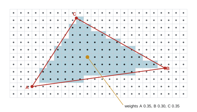
The edge functions do more than test coverage. Dividing each by the triangle's total signed area gives the barycentric coordinates \((\lambda_A, \lambda_B, \lambda_C)\) of the point: \(\lambda_A = E_{BC}(p)/E_{AB}(C)\) and so on. They are non-negative inside the triangle and sum to one, and any quantity defined at the vertices, such as color, depth, texture coordinates or normals, can be interpolated across the triangle as \(\lambda_A f_A + \lambda_B f_B + \lambda_C f_C\). Henri Gouraud's 1971 smooth shading did exactly this with colors. In perspective, attributes must be interpolated in a perspective-correct way, which lesson 9 explains.
# Triangle rasterization with edge functions and barycentric coordinates.
# Each pixel middle is tested against three edges; covered pixels show which
# vertex dominates their shade by barycentric weight (A, B or C).
def edge(a, b, p):                    # twice the signed area of triangle (a, b, p)
    return (b[0] - a[0]) * (p[1] - a[1]) - (b[1] - a[1]) * (p[0] - a[0])
A, B, C = (2.0, 1.0), (21.0, 4.0), (8.0, 11.0)     # counter-clockwise
area = edge(A, B, C)
W, H = 24, 12
rows, inside, check = [], 0, []
for y in range(H):
    row = ''
    for x in range(W):
        p = (x + 0.5, y + 0.5)                    # sample at the pixel middle
        w0, w1, w2 = edge(B, C, p), edge(C, A, p), edge(A, B, p)
        if w0 >= 0 and w1 >= 0 and w2 >= 0:       # inside (top-left rule omitted here)
            l = (w0 / area, w1 / area, w2 / area)  # barycentric weights of A, B, C
            row += 'ABC'[max(range(3), key=lambda i: l[i])]; inside += 1
            if (x, y) == (10, 5): check = l
        else:
            row += '.'
    rows.append(row)
for r in reversed(rows): print(r)
print(f"area = {area / 2} square pixels, covered pixel midpoints = {inside}")
print("weights at pixel (10, 5):", tuple(round(v, 3) for v in check), "sum", round(sum(check), 6))........................ ........C............... .......CCCC............. ......CCCCCCC........... ......CCCCCCCCB......... .....CCCCCCCCBBB........ .....AAAACCBBBBBBB...... ....AAAAAAABBBBBBBBB.... ...AAAAAAAABBBBBBB...... ...AAAAAAAAA............ ..AAA................... ........................ area = 86.0 square pixels, covered pixel midpoints = 88 weights at pixel (10, 5): (0.314, 0.337, 0.349) sum 1.0
The covered pixels form the triangle's discrete footprint, labeled by whichever vertex has the largest barycentric weight, so the image partitions into three regions around the vertices. The printed weights at one pixel are all positive and sum to one. The number of covered pixel centers is close to the triangle's area in pixels, as it should be on average.
Two triangles that share an edge raise a subtle problem. A pixel center lying exactly on the shared edge would be counted by both triangles, drawing it twice (wrong for transparent blending) or by neither (leaving a crack). Graphics APIs therefore specify a tie-breaking fill rule. Direct3D and most other APIs use the top-left rule: a sample exactly on an edge is inside only if the edge is a top edge (horizontal and above the other vertices) or a left edge. Implementations also snap vertex positions to a fixed-point sub-pixel grid, typically with 8 bits of fraction, so that the edge tests are exact and consistent across triangles. Watertight rasterization, with no cracks and no double coverage, is a hard requirement of every graphics API.
Sampling and aliasing
Rasterization samples a continuous image at discrete points, and sampling theory explains what goes wrong. The Nyquist–Shannon sampling theorem says that a signal containing no frequencies above B can be perfectly reconstructed from samples taken at a rate above 2B. A geometric edge is a step, which contains arbitrarily high frequencies, so no sampling rate is enough. Frequencies above half the sampling rate do not simply disappear; they fold back and masquerade as lower frequencies. This is aliasing. In images it appears as jagged staircase edges (jaggies), as moiré patterns on fine repetitive detail such as fences or fabric, and in animation as crawling edges and shimmering highlights, often more objectionable than the still artifacts.
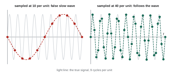
There are two cures in principle: sample at a higher rate, or remove the high frequencies before sampling (prefiltering). For an edge, prefiltering means computing the exact fraction of each pixel area covered by the shape, convolved with a filter, and using that as the pixel's coverage. That is expensive for general scenes, so practical antialiasing approximates it with more samples per pixel and a reconstruction filter that averages them.
Antialiasing techniques
Supersampling antialiasing (SSAA) renders the image at a higher resolution, for example with four or sixteen samples per pixel, and averages the samples into each final pixel. It handles every kind of aliasing, from geometric edges to texture and shading, but its cost scales with the number of samples. Sample placement matters: a regular grid aligns badly with near-horizontal and near-vertical edges, so rotated-grid and stratified or jittered patterns give better quality per sample. With n samples per pixel, an edge can show at most \(n + 1\) intensity levels.
# Aliasing and supersampling: estimate how much of each pixel a thin diagonal
# stripe covers using 1, 4 (2x2 grid) and 16 (4x4 grid) samples per pixel.
import math
def covered(x, y):                    # a stripe of width 0.6 along y = 0.45 x + 1
    d = abs(0.45 * x - y + 1) / math.hypot(0.45, 1)
    return d < 0.3
def pixel_value(px, py, n):           # n x n regular grid of samples
    hits = sum(covered(px + (i + 0.5) / n, py + (j + 0.5) / n) for i in range(n) for j in range(n))
    return hits / (n * n)
def exact(px, py, m=200):             # reference: a very dense grid
    return pixel_value(px, py, m)
shades = ' .:-=+*#%@'
for n in (1, 2, 4):
    err = 0.0
    lines = []
    for py in range(5, -1, -1):
        s = ''
        for px in range(12):
            v = pixel_value(px, py, n); err += abs(v - exact(px, py, 60))
            s += shades[min(9, int(v * 9.999))]
        lines.append(s)
    print(f"{n * n:2} sample(s) per pixel, mean absolute coverage error {err / 72:.3f}")
for s in lines: print(' |' + s + '|')1 sample(s) per pixel, mean absolute coverage error 0.082 | @@ | | @@ | | @ | | @ | |@@ | | | 4 sample(s) per pixel, mean absolute coverage error 0.022 | :==:| | :#= | | :== | | =#: | |=#: | | | 16 sample(s) per pixel, mean absolute coverage error 0.007 | .**.| | :*= | | -*- | | =*- | |++. | |. |
With one sample per pixel the stripe is either fully on or off in each pixel and appears broken and stair-stepped; with 4 and then 16 samples, partial coverage shows as intermediate shades, and the mean error against a dense reference falls sharply. The printed shades are a rough approximation of what the eye sees: a smoother, continuous stripe.
Multisample antialiasing (MSAA), standard in GPUs since the early 2000s, exploits the observation that geometric aliasing at triangle edges is usually the worst problem. It stores several coverage and depth samples per pixel, typically 4 or 8, but runs the expensive pixel shader only once per pixel per triangle and copies the result to the covered samples. Edges get smooth coverage for a fraction of the cost of supersampling, but aliasing inside triangles, from textures or sharp specular highlights, is not addressed.
Deferred rendering engines, which shade after rasterizing all geometry (lesson 6), work poorly with MSAA, and the industry turned to post-processing and temporal methods. Morphological antialiasing (MLAA, 2009) and fast approximate antialiasing (FXAA, 2009) detect edges in the finished image and blend across them, which is cheap but can blur detail. Temporal antialiasing (TAA), now the default in most game engines, jitters the projection by a sub-pixel offset each frame and blends the new frame with a history buffer reprojected using motion vectors, accumulating many samples over time. TAA handles all kinds of aliasing at low cost, but can produce ghosting and blur when the history is wrong, which engines fight with history rejection heuristics. Machine-learning upscalers such as NVIDIA's DLSS, AMD's FSR 4 and Intel's XeSS extend temporal accumulation: they render at a lower resolution and reconstruct a higher-resolution antialiased image, which lesson 12 discusses.
| Technique | Idea | Strengths | Weaknesses |
|---|---|---|---|
| SSAA | Render and shade many samples per pixel, then average | Handles all aliasing | Cost multiplies with sample count |
| MSAA | Many coverage and depth samples, one shade per pixel per triangle | Smooth geometric edges at modest cost | No help inside triangles; awkward with deferred shading |
| FXAA, MLAA, SMAA | Find edges in the final image and blend | Very cheap, works with any renderer | Blurs fine detail; misses sub-pixel features |
| TAA | Jitter each frame and accumulate a reprojected history | Handles all aliasing cheaply | Ghosting and blur when reprojection fails |
| ML upscaling | Learned temporal reconstruction from lower resolution | High quality at reduced render cost | Vendor-specific; can hallucinate or smear detail |
Worked examples
Worked problem
Edge function test
For the triangle A = (0, 0), B = (8, 0), C = (0, 6), is the point p = (3, 2) inside? Give its barycentric coordinates.
Show solution
- Total: \(E_{AB}(C) = (8-0)(6-0) - (0-0)(0-0) = 48\).
- \(E_{BC}(p) = (0-8)(2-0) - (6-0)(3-8) = -16 + 30 = 14\).
- \(E_{CA}(p) = (0-0)(2-6) - (0-6)(3-0) = 0 + 18 = 18\).
- \(E_{AB}(p) = (8-0)(2-0) - (0-0)(3-0) = 16\). All are non-negative, so p is inside.
- Barycentric: \(\lambda_A = 14/48 = 0.292\), \(\lambda_B = 18/48 = 0.375\), \(\lambda_C = 16/48 = 0.333\); they sum to 1.
Answer: Inside, with weights (0.292, 0.375, 0.333) for A, B and C.
Worked problem
Nyquist and a picket fence
A fence in the distance has 40 pickets across 100 pixels of screen. With one sample per pixel, will it alias?
Show solution
- The pattern has 40 cycles over 100 pixels, a frequency of 0.4 cycles per pixel.
- The sampling rate is 1 sample per pixel, so the Nyquist limit is 0.5 cycles per pixel.
- At 0.4 cycles per pixel the pattern is below the limit, but close; pickets have sharp edges whose harmonics (0.8, 1.2 cycles per pixel) exceed it.
Answer: The fundamental is representable, but the sharp edges alias, and as the fence recedes past 50 pickets per 100 pixels the whole pattern aliases into moiré.
Worked problem
MSAA cost
A frame at 1920 by 1080 uses 4x MSAA. How many depth samples are stored, and roughly how many pixel shader invocations occur compared with 4x SSAA?
Show solution
- Depth samples: \(1920 \times 1080 \times 4 = 8{,}294{,}400\).
- MSAA shades about once per pixel per covering triangle, plus extra at edges where several triangles share a pixel; SSAA shades all 8.3 million samples.
- Typically MSAA runs a little over a quarter as many shader invocations as 4x SSAA.
Answer: About 8.3 million depth samples; shading cost is close to non-antialiased rendering rather than four times it.
Common mistakes
MistakeTest pixel corners against triangle edges.
InsteadSample at pixel centers (x + 0.5, y + 0.5) consistently, as graphics APIs specify.
MistakeLet pixels on shared edges be drawn by both triangles.
InsteadApply a consistent fill rule such as the top-left rule, with snapped fixed-point vertex positions.
MistakeThink that more resolution eliminates aliasing.
InsteadEdges contain unbounded frequencies; higher resolution reduces but cannot remove aliasing without filtering.
MistakeExpect MSAA to fix shimmering textures and specular highlights.
InsteadMSAA only antialiases coverage at triangle edges; texture filtering and temporal methods handle the rest.
MistakeInterpolate attributes linearly in screen space for perspective views.
InsteadUse perspective-correct interpolation (lesson 9).
Summary and key terms
- Rasterization finds the pixels covered by a primitive; GPUs do it in dedicated hardware.
- Bresenham's algorithm draws lines with integer arithmetic, one pixel per step along the major axis.
- Edge functions test whether a sample lies inside a triangle and give barycentric coordinates for interpolation.
- Fill rules such as the top-left rule and fixed-point snapping make rasterization watertight.
- Aliasing occurs when a signal contains frequencies above half the sampling rate; edges always do.
- Supersampling, multisampling, post-process filters and temporal accumulation trade quality against cost.
- Temporal antialiasing and learned upscalers dominate modern real-time rendering.
- Rasterization
- Converting geometric primitives into the set of pixels or samples they cover.
- Bresenham's algorithm
- An integer-only incremental algorithm for drawing lines.
- Edge function
- A linear function whose sign tells which side of a directed edge a point lies on.
- Barycentric coordinates
- Weights expressing a point in a triangle as a combination of its vertices.
- Fill rule
- A tie-breaking convention deciding which triangle owns samples exactly on shared edges.
- Aliasing
- Artifacts caused by sampling a signal with frequencies above half the sampling rate.
- Nyquist rate
- Twice the highest frequency in a signal, the minimum rate for exact reconstruction.
- Supersampling
- Taking and averaging several samples per pixel.
- MSAA
- Multisample antialiasing: several coverage samples per pixel with one shading evaluation per triangle.
- Temporal antialiasing
- Accumulating jittered samples over frames using reprojection.
Practice problems
Work each problem on paper first, then reveal the answer to check.
How many pixels does Bresenham draw for a line from (0, 0) to (10, 3)?
Show answer
11, one per column along the major axis.
Why do GPUs prefer edge functions to scanline filling?
Show answer
Each sample can be tested independently and incrementally, which suits parallel hardware.
What is the sign of the edge function for points to the left of a counter-clockwise edge?
Show answer
Positive.
What do barycentric coordinates sum to?
Show answer
One.
What problem does the top-left rule solve?
Show answer
Samples on edges shared by two triangles being drawn twice or not at all.
A pattern repeats every 1.5 pixels. Can it be sampled at one sample per pixel without aliasing?
Show answer
No: its frequency is 0.67 cycles per pixel, above the 0.5 limit.
How many intensity levels can an edge show with 4 samples per pixel?
Show answer
Five, from 0 to 4 covered samples.
What does MSAA share across samples to save cost?
Show answer
The pixel shader result for each triangle.
What artifact is typical of temporal antialiasing?
Show answer
Ghosting or blur when the reprojected history is wrong.
Why are vertex positions snapped to a sub-pixel grid?
Show answer
So edge tests are exact and consistent across adjacent triangles.
Lesson quiz · 5 questions
Score 60% or more to complete this lesson.
Create a free account to save your progress, take quizzes and earn a certificate.