Envelope and systems inputs

Holm hands each student a sheet with the inputs Sethi used in the hub's model last year: wall and roof constructions, window properties, airtightness, ventilation rates, lighting and plug load densities, heat pump curves, setpoints and schedules. Beside each value is a blank column headed 'How sure?'. 'Fill it in,' he says. 'For each input, write the range within which you are confident the real building will fall.' The students work through the list. The wall's thermal resistance they can bound tightly; the window U-value fairly tightly; the airtightness only within a factor of three or four until the building is tested; the plug loads of a daycare and a community kitchen hardly at all. Holm collects the sheets. 'Now you know where the model's real uncertainty lies. Today we find out which of those uncertainties actually matter.'

Envelope inputs

The envelope inputs describe how each construction conducts, stores and transmits heat and light. For opaque constructions the model needs each layer's thickness, conductivity, density and specific heat, or an equivalent overall U-value with its mass, and the solar absorptance and thermal emittance of the outer and inner surfaces. The students learned in Building Envelope and Detailing that the nominal resistance of the insulation is not the effective resistance of the assembly: studs, clips, slab edges, balconies and window frames create thermal bridges that can reduce the effective value of a wall by a third or more. The model must use effective values, either by derating the clear-field U-value with linear and point transmittances, as the students did with psi-values, or by modeling the bridges explicitly.

Windows need more detail than walls: the U-value of the whole window including frame, the solar heat gain coefficient (SHGC), the visible transmittance, and the geometry of frames and dividers. Many engines also accept a full optical description of each pane, which matters for daylight and for angular effects. The hub's triple-glazed windows have a whole-window U of about 0.14 Btu/h·ft²·°F, an SHGC of about 0.40 and a visible transmittance of about 0.55. Holm warns that values from the window schedule are often center-of-glass values, which are better than the whole-window values the model needs.

Airtightness and infiltration

Air leakage is the most uncertain envelope input. Before construction, the modeler must assume a value; after construction, a blower door test measures it, as the students did at the hub in Building Envelope and Detailing. Test results are reported at a pressure of 50 or 75 Pa, far above the pressures that act on a building most of the time, so they must be converted to an infiltration rate under normal conditions. Simple rules divide the air changes at 50 Pa by about 20 to estimate natural air changes; better methods calculate infiltration hour by hour from wind and stack effect, using the measured leakage curve. For a building with a very tight envelope and balanced ventilation, infiltration is small and its uncertainty matters little; for an ordinary building it can be one of the largest loads.

Internal loads and schedules

People, lighting and equipment add heat and use energy. Lighting power density is set by the design and can be bounded well; occupancy and plug loads cannot. The energy used by computers, kitchen equipment, a daycare's laundry and the hall's audiovisual system depends on choices that are not yet made and on how people will behave. Standards give default densities for compliance; measured studies of real buildings show wide spreads around them. For a building aiming at net zero, where heating has been squeezed down by a superb envelope, plug loads often become the largest end use, as the students found in Sustainable and Regenerative Design.

Systems inputs

System inputs include the type and arrangement of equipment, capacities, efficiencies and their performance curves, fan power, pump power, control sequences and setpoints. As Lesson 3 showed, the most important are often the controls: setpoints, setback, economizer operation, demand-controlled ventilation, and the temperatures at which heat pumps switch to backup heat. Heat recovery effectiveness, typically 0.75 to 0.90 for good heat recovery ventilators, has a large effect in a cold climate, and real effectiveness is often lower than the rated value because of frost control and imbalance between supply and exhaust flows.

Sensitivity analysis

A sensitivity analysis asks how much the result changes when the inputs change. Its purpose is practical: to find the few inputs that matter, so that the team can pin them down, design them out, or at least report the uncertainty they create. Holm introduces three methods, in order of effort.

• One at a time: change each input from its low to its high value while holding the others at their base values, and record the change in the result. Simple and transparent, but it misses interactions, where the effect of one input depends on another.
• Screening by the method of Morris: take random paths through the input space, changing one input at a time along each path, and average the size of each input's effect over many paths. The mean of the absolute effects, written mu-star, ranks importance; their spread, sigma, reveals non-linear effects and interactions.
• Global variance-based methods such as Sobol indices: sample the whole input space and divide the variance of the result among the inputs and their interactions. Thorough but expensive, often thousands of runs, usually done with a surrogate model, as Lesson 12 describes.

The students apply the Morris method to a quick stand-in for the hub's energy model, with seven inputs varied over the ranges they wrote on their sheets. Each of twenty paths changes all seven inputs once, so the screening takes 160 model runs: affordable even with a real engine running overnight.

# Which inputs matter? A screening of the hub's energy model by the method of Morris
import random
random.seed(5)
inputs = {   # label shown: (low, high) in SI units used inside the model
    "wall R-28 to R-51": (5.0, 9.0),        # wall thermal resistance, m2K/W
    "window U 0.12 to 0.28": (0.7, 1.6),        # window U, W/m2K
    "airtightness ACH50": (0.6, 3.0),
    "heat recovery": (0.60, 0.90),
    "lighting 0.28 to 0.65 W/ft2": (3.0, 7.0),        # lighting power density, W/m2
    "plug loads 0.37 to 1.1 W/ft2": (4.0, 12.0),       # plug load density, W/m2
    "setpoint 66 to 73 F": (19.0, 23.0),      # heating setpoint, C
}
names = list(inputs)
def eui(x):
    """A quick stand-in for the hub's energy model: kWh per m2 per year."""
    wall, win, ach, hr, lpd, plug, sp = x
    ua = 1300 / wall + 600 * win + 60 * ach + 1800 * (1 - hr) * 0.33   # W/K
    hdd = 4300 * (1 + 0.09 * (sp - 21))
    heat = ua * hdd * 24 / 1000 / 2458 - 0.8 * (lpd + plug) * 1.1          # internal gains offset heat
    return max(heat, 0) / 2.4 + lpd * 2.6 + plug * 3.0 + 8
def scale(u):
    return [inputs[n][0] + ui * (inputs[n][1] - inputs[n][0]) for n, ui in zip(names, u)]
levels, delta = 4, 2 / 3
effects = {n: [] for n in names}
for r in range(20):                                   # twenty trajectories through the input space
    u = [random.choice([0, 1 / 3]) for _ in names]
    y = eui(scale(u))
    for k in random.sample(range(len(names)), len(names)):
        u2 = list(u); u2[k] += delta
        y2 = eui(scale(u2))
        effects[names[k]].append((y2 - y) / delta)
        u, y = u2, y2
rows = []
for n in names:
    e = effects[n]
    mu_star = sum(abs(v) for v in e) / len(e)
    mean = sum(e) / len(e)
    sd = (sum((v - mean) ** 2 for v in e) / (len(e) - 1)) ** 0.5
    rows.append((mu_star, sd, n))
for mu_star, sd, n in sorted(rows, reverse=True):
    print(f"{n:20s} mu* {mu_star * 0.317:5.1f}   sigma {sd * 0.317:4.1f}  (kBtu/ft2 across the range)")

plug loads 0.37 to 1.1 W/ft2 mu*   6.7   sigma  0.0  (kBtu/ft2 across the range)
window U 0.12 to 0.28 mu*   3.1   sigma  0.4  (kBtu/ft2 across the range)
lighting 0.28 to 0.65 W/ft2 mu*   2.8   sigma  0.0  (kBtu/ft2 across the range)
setpoint 66 to 73 F  mu*   2.3   sigma  0.3  (kBtu/ft2 across the range)
heat recovery        mu*   1.0   sigma  0.1  (kBtu/ft2 across the range)
airtightness ACH50   mu*   0.8   sigma  0.1  (kBtu/ft2 across the range)
wall R-28 to R-51    mu*   0.6   sigma  0.1  (kBtu/ft2 across the range)

The ranking is clear. Plug loads dominate, with an effect of about 6.7 kBtu/ft² across their range, followed by window U, lighting and the setpoint. Heat recovery and airtightness matter much less, and the wall's thermal resistance, between R-28 and R-51, matters least of all, about 0.6 kBtu/ft². The sigma of plug loads and lighting is zero because in this simple model their effect is the same everywhere; the window, setpoint and envelope inputs interact with one another and with the climate, so their effects vary from path to path.

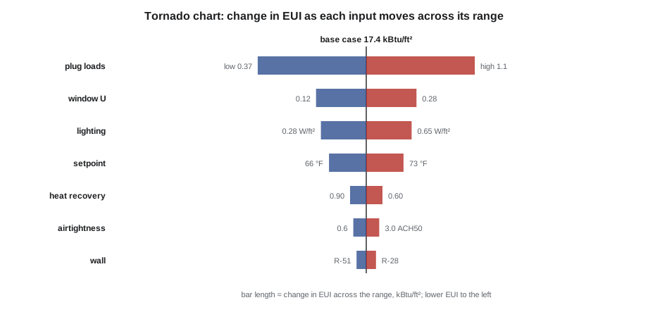
Ingrid draws two conclusions that Holm wants the whole class to hear. First, for this building, further insulation of the walls is nearly pointless in energy terms; the money and carbon would be better spent elsewhere. Second, the largest uncertainty in the net-zero claim is not in anything the architects are drawing: it is in how the hub's users will run their equipment. The response is not to give up but to act on the uncertainty: specify efficient appliances, meter plug loads separately, give the operators feedback, and size the roof array with a margin for the high end of the plug load range.

Inputs and the ranges behind them

Sensitivity results depend entirely on the ranges chosen. A narrow range makes an input look unimportant; a wide one makes it look dominant. Ranges should reflect genuine uncertainty at the current stage of design, drawn from sources the team can defend: manufacturers' data with tolerances, measured studies of similar buildings, field test results, and the judgment of experienced operators. As the design advances, ranges narrow: the walls are detailed, the windows chosen, the airtightness tested. Repeating the sensitivity analysis at each stage keeps the team's attention on the inputs that still matter.

Holm also distinguishes two kinds of input. Design parameters are choices the team makes, such as wall resistance or window type; for these, sensitivity analysis shows which choices are worth studying. Uncertain parameters are things the team cannot control, such as occupant behavior or future weather; for these, it shows how robust the design is. A good design is one that performs well across the plausible range of the uncertain parameters, not one that is optimal only at their assumed values.

Defaults, libraries and their dangers

Every simulation tool comes with libraries of constructions, schedules and equipment. They are convenient and dangerous. A library wall may have the right nominal resistance but omit thermal bridges; a library schedule may assume an office that closes at five; a library heat pump may have a performance curve measured in a mild climate. Sethi's rule is that every library item used in a model must be opened, read and either accepted or changed, and the decision recorded. 'The software does not know your building. Neither does whoever made the library.'

Exercise 5: sensitivity of the hub

Each student runs a screening sensitivity analysis on their hub model.

• Choose at least eight inputs and write down a defended range for each.
• Run a one-at-a-time analysis and draw a tornado chart.
• Run a Morris screening with at least ten paths and compare the ranking.
• Identify which inputs are design parameters and which are uncertain parameters.
• Recommend actions for the three most important uncertain parameters.

Self-critique checklist

• Is every range defended by a source?
• Have I used effective rather than nominal envelope values?
• Have I opened and checked every library item I used?
• Do my recommendations address the uncertainties that matter most?