
ARCH-510 · Lesson 12 of 12 · 22 min
Simulation project
The last four weeks of the term belong to the simulation project. Each student takes one building through a complete performance study, from the question to the report, using every method of the course. Wren studies her thesis site, a school on a river bank; Ingrid studies a seniors' residence for a housing co-operative; Joon-ho studies a library he is designing for his thesis. Callum, who has always been the most doubtful of the four about simulation, takes the building the class knows best: the community hub, in its net-zero design. 'If our models are going to be wrong anywhere,' he says, 'I want to find out where on a building we have argued about for three years.' This lesson follows his project.
The brief
Callum's brief, agreed with Holm and with the city's facilities department as a mock client, asks four questions, each tied to a decision.
- Is the hub net-zero operational carbon over a year, and how confident can the city be? Decision: the size of the roof array and the plug load policy.
- Will the reading room work as a neighborhood cool room in a 2050s heat wave? Decision: whether to add mechanical cooling to the reading room's heat pumps.
- Do the reading room and playrooms have good daylight without disturbing glare? Decision: the fins, the shading of the playrooms and the reading room layout.
- How robust is the upfront carbon budget? Decision: whether to specify the low-carbon concrete mix.
He agrees metrics and criteria for each question before running any model, and records them on the first page of the report: annual net balance and the share of plausible runs with a positive balance; hours above the adaptive 80 limit during a 2050s heat-wave week and a health limit of 86 °F for the cool room; sDA300/50, ASE1000,250 and glare autonomy at the reading desks and nap positions; and the median and range of upfront carbon, with the share of draws in which the low-carbon mix is better.
The models
Callum builds three linked models from the same geometry. The energy model has fourteen zones, following the zoning of Lesson 4, an airflow network for the hall and reading room, heat pump curves from the manufacturer covering the full range of outdoor temperature, and backup heat. The daylight model, in Radiance, has measured reflectances of the specified finishes and six ambient bounces, and passes hourly lighting schedules to the energy model. The LCA uses the bill of materials checked against the structural and architectural drawings, with product-specific EPDs where the suppliers have them. An input log records every value and its source; Sethi reviews it and finds two errors, a window frame value and a library schedule for the daycare, which Callum corrects.
He checks every model as Lesson 3 taught: the design heating load against a hand calculation, a winter and a summer week plotted and explained, unmet hours below fifty a year, an EUI within the range of published values for Passive House community buildings, and a daylight result compared with the simple daylight factor calculation from Environmental Systems I.
Uncertainty and the surrogate
To answer the net-zero question with confidence, Callum needs hundreds of runs with the uncertain inputs varied together: plug loads, hall use, setpoints, airtightness after construction, heat pump performance, snow cover on the array and the weather. Each full run of the energy model takes about three minutes, so five hundred runs would take a day. That is affordable once, but not every time the design changes. His solution, increasingly common in practice and research, is a surrogate model: a fast statistical model trained on a modest number of full runs, which can then be evaluated thousands of times in seconds.
Surrogates range from straight-line regressions to Gaussian processes and neural networks. Since the mid-2020s, machine-learning surrogates trained on large libraries of simulations have been built into design tools, giving architects near-instant feedback while they draw. Holm treats them with the same discipline as any model: a surrogate is only as good as the runs it was trained on, it must be tested on runs it has not seen, and it must never be used outside the range of inputs it was trained on. The students write the simplest possible surrogate, a linear regression on three inputs fitted to forty runs of a stand-in model, and test it.
# A surrogate for the hub's energy model: fit a straight-line model to 40 simulation runs, then test it
import random
random.seed(12)
def simulate(wwr, rsi, plug):
    """Stand-in for one full simulation run: EUI in kWh/m2 (with a little curvature the line cannot capture)."""
    heat = (1300 / rsi + 2200 * wwr * 0.8 + 900) * 4300 * 24 / 1000 / 2458 / 2.6
    light = 14.0 - 24.0 * min(wwr, 0.32)
    return heat - 170 * wwr * 0.35 * 2200 / 2458 / 2.6 + light + 3.0 * plug + 8
def sample():
    return [random.uniform(0.15, 0.45), random.uniform(5.0, 10.0), random.uniform(4.0, 10.0)]
train = [sample() for _ in range(40)]
y = [simulate(*x) for x in train]
X = [[1.0] + x for x in train]
# least squares by the normal equations, solved with Gaussian elimination
k = len(X[0])
A = [[sum(r[i] * r[j] for r in X) for j in range(k)] + [sum(r[i] * t for r, t in zip(X, y))] for i in range(k)]
for i in range(k):
    piv = A[i][i]
    A[i] = [v / piv for v in A[i]]
    for j in range(k):
        if j != i:
            f = A[j][i]; A[j] = [a - f * b for a, b in zip(A[j], A[i])]
coef = [A[i][k] for i in range(k)]
def predict(x):
    return coef[0] + sum(c * v for c, v in zip(coef[1:], x))
test = [sample() for _ in range(200)]
err = [abs(predict(x) - simulate(*x)) for x in test]
yt = [simulate(*x) for x in test]; mean = sum(yt) / len(yt)
r2 = 1 - sum((predict(x) - t) ** 2 for x, t in zip(test, yt)) / sum((t - mean) ** 2 for t in yt)
print("surrogate, EUI in kWh/m2 = {:.1f} {:+.1f} x window share {:+.2f} x wall RSI {:+.2f} x plug W/m2".format(*coef))
print(f"tested on 200 new runs: R2 {r2:.3f}, mean error {sum(err) / len(err) * 0.317:.2f} kBtu/ft2, worst {max(err) * 0.317:.2f} kBtu/ft2")
x = [0.30, 20.0, 6.0]                                 # far outside the range the surrogate was trained on
print(f"outside the training range (RSI 20): surrogate {predict(x) * 0.317:.1f}, simulation {simulate(*x) * 0.317:.1f} kBtu/ft2")surrogate, EUI in kWh/m2 = 39.9 -6.9 x window share -0.36 x wall RSI +3.04 x plug W/m2 tested on 200 new runs: R2 0.990, mean error 0.14 kBtu/ft2, worst 0.41 kBtu/ft2 outside the training range (RSI 20): surrogate 15.5, simulation 16.1 kBtu/ft2
Fitted to forty runs, the straight-line surrogate reproduces two hundred new runs with an R² of about 0.99 and an average error of about 0.14 kBtu/ft², at a tiny fraction of the cost. Outside the range it was trained on, at a wall of RSI 20, it misses by about 0.6 kBtu/ft², half again its worst error inside the range, because the true effect of insulation flattens out while the straight line keeps falling. Callum's own surrogate, a Gaussian process trained on eighty full runs of the hub model with seven inputs, reproduces held-out runs within about 2 in 100, and he uses it only within the ranges of its training data.
Results
Callum's report opens with a one-page dashboard: each question, its metric and criterion, the result with its range, and the decision it supports.
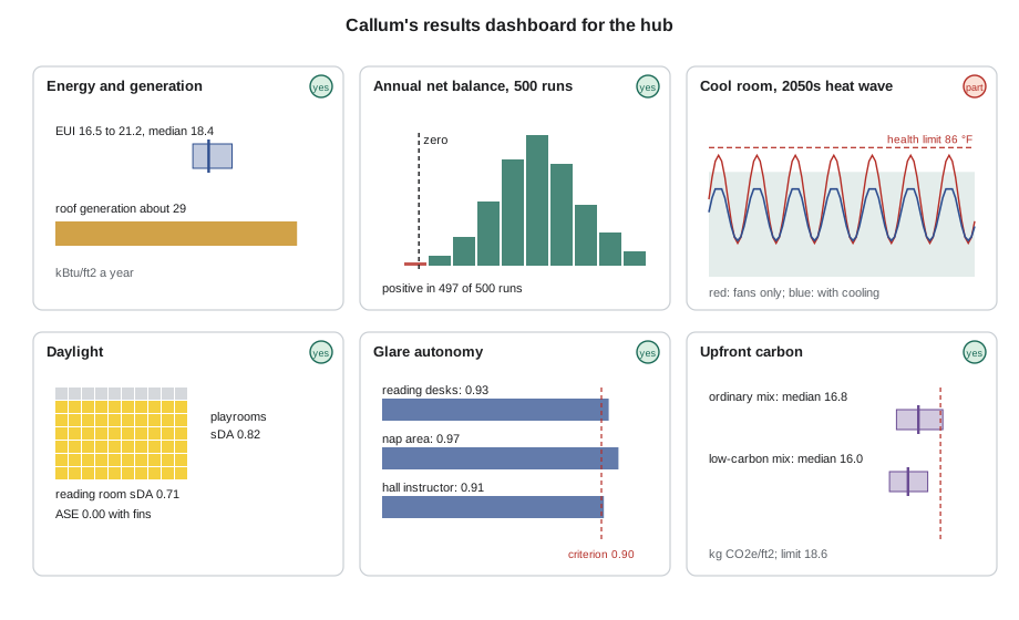
| Question | Criterion | Result | Met? |
|---|---|---|---|
| Net-zero operational carbon | Positive balance in at least 95 of 100 plausible runs | EUI median 18.4 kBtu/ft², range 16.5 to 21.2; generation about 29.0 kBtu/ft²; positive in 497 of 500 runs | Yes |
| Cool room, 2050s heat wave | No occupied hour above the health limit; few above the adaptive limit | Fans and night ventilation: 6 of 84 hours above adaptive limit, peak 85 °F; with heat pump cooling on 3 days: 0 hours, peak 80 °F | Only with cooling |
| Reading room daylight | sDA300/50 at least 0.55 | 0.71 | Yes |
| Reading room sun | ASE1000,250 at most 0.10 | 0.00 with fins | Yes |
| Glare at reading desks | Glare autonomy at least 0.90 | 0.93 with desks turned to the side | Yes |
| Upfront carbon | Median below 18.6 kg CO₂e/ft² | Median 16.0 with low-carbon mix, range 14.5 to 17.6 | Yes |
The net-zero claim holds: in 497 of 500 plausible runs the roof array produces more than the hub uses. The three failures combine the highest plug loads with a winter of long snow cover on the array; Callum recommends a plug load policy, metering of the hall's equipment and a snow-clearing plan for the lower roof rather than more panels. The cool room question is answered honestly: fans and night ventilation keep the reading room below the health limit but not within the adaptive band on the hottest afternoons, so he recommends enabling cooling from the existing heat pumps for the few worst days, with the electricity covered by the array. The fins bring ASE to zero, and the energy model shows they cost less than 1 in 100 of the reading room's winter solar gain, so he recommends them. With product-specific EPDs and shared items drawn once, the low-carbon concrete mix is better in 498 of 500 draws.
Presenting results
Holm spends a seminar on how to present simulation to people who will not read the report. His rules are short.
- Lead with the decision, not the method. 'The array is large enough; adopt a plug load policy' comes first; the surrogate comes later.
- Show ranges, not just numbers, and say what the range means in plain words: 'in 497 of 500 plausible futures'.
- Use one chart per question, with the criterion drawn on it.
- Report what was not met as clearly as what was.
- Say what each model left out and what would change the answer.
- Keep the input log and the model files so that anyone can check the work.
He adds that the architect's role in a simulation project is to keep the questions architectural. Simulation can say how much daylight a monitor brings; only the architect can say whether a reading room under that light, with those shadows and that view, is a good place to read.
The review
The final review brings back people who have taught the students over five years: Sethi; Professor Ruth Abernathy, who taught Environmental Systems I; Mei Takahashi; and Professor Tobias Reinholt, who led the net-zero studio. Abernathy asks Callum whether the energy model could be checked once the hub is built. He shows his measurement and verification plan: sub-meters on the heat pumps, the lighting, the hall's equipment and the daycare kitchen; temperature loggers in five rooms; a blower door test at completion; and a calibration of the model against the first year's interval data, using the Guideline 14 hourly criteria. Takahashi asks whether the LCA will be updated with the as-built quantities and actual EPDs; it will. Reinholt asks the hardest question: after three years of argument, what did the full simulation change? Callum answers without hesitation: it found that the heat-wave strategy needed mechanical cooling for a few days, that the net-zero margin depends on plug loads rather than on the envelope, and that the reading room's layout matters more for glare than its shading. 'None of those were in our spreadsheets.'
Holm closes the course with the loop from Lesson 1. 'You have learned to frame a question, build the simplest model that can answer it, check it, test its sensitivity, attach uncertainty to it and present it honestly. When your buildings are built, measure them, and compare the measurements with what you predicted. That comparison is how the profession learns.'
Worked problem
Writing the executive summary
Callum must summarize his project on half a page for the city's facilities manager, who will not read the rest. What should the summary contain?
Show solution
- The four decisions, each with its recommendation in one sentence.
- For each, the result that supports it, with its range in plain words.
- What is not met and what is proposed instead.
- The main uncertainties and how the measurement plan will address them.
- A sentence on what the models leave out.
Answer: The summary reads: the roof array is large enough for net zero in 497 of 500 plausible cases, provided a plug load policy is adopted; the reading room needs cooling on a few days a year to serve as a cool room in the 2050s; the fins should be built; the low-carbon mix should be specified; and the building should be metered and the model calibrated in its first year.
Exercise 12: the simulation project
Each student completes a simulation project on a building of their choice.
- Write a brief with questions, decisions, metrics and criteria agreed in advance.
- Build and check energy, daylight and LCA models from shared geometry, with an input log.
- Test sensitivity and propagate uncertainty, using a tested surrogate if needed.
- Present a one-page dashboard and an executive summary, with what was and was not met.
- Prepare a measurement and verification plan.
Self-critique checklist
- Is every result tied to a decision and a criterion?
- Has every model been checked, and every input logged?
- Have I reported ranges and what drives them?
- Have I said what the models leave out?
Common mistakes
MistakeLeading the presentation with the method.
InsteadLead with the decisions and the results that support them.
MistakeUsing a surrogate outside the range it was trained on.
InsteadTest it on unseen runs and use it only within its training range.
MistakeHiding criteria that were not met.
InsteadReport them clearly, with the reasons and the proposed response.
MistakeEnding the study at handover.
InsteadPlan measurement and calibration after occupancy.
MistakeLetting simulation replace architectural judgment.
InsteadUse it to inform decisions whose architectural meaning the designer must still judge.
Summary and key terms
- A simulation project starts with questions tied to decisions, with metrics and criteria agreed in advance.
- Linked energy, daylight and LCA models built from shared geometry, with an input log and checks, provide the evidence.
- Surrogate models make large uncertainty studies affordable, but must be tested and used only within their training range.
- Results are presented as decisions supported by ranges, with unmet criteria reported as clearly as met ones.
- Measurement and calibration after occupancy close the performance-based design loop.
- Simulation brief
- A statement of the questions, decisions, metrics and criteria a study must address.
- Surrogate model
- A fast statistical model trained on full simulation runs.
- Gaussian process
- A flexible statistical model often used as a surrogate, which also estimates its own uncertainty.
- Training range
- The range of inputs covered by the runs a surrogate was trained on.
- R²
- The share of variation in the results explained by a model.
- Dashboard
- A one-page summary of questions, criteria and results.
- Executive summary
- A short summary for decision makers, leading with recommendations.
- M and V plan
- A measurement and verification plan for checking performance after occupancy.
Practice problems
Work each problem on paper first, then reveal the answer to check.
Why test a surrogate on runs it was not trained on?
Show answer
To check that it predicts new cases, not just the training data; a model can fit its training runs well and still predict poorly.
Why did the straight-line surrogate miss badly at RSI 20?
Show answer
The true effect of insulation flattens at high values, but the straight line keeps falling; RSI 20 was outside the training range.
The net balance is positive in 497 of 500 runs. How would you explain this to a client?
Show answer
In almost every plausible combination of use, weather and equipment performance, the hub produces more energy than it uses; the few exceptions combine very high plug loads with long snow cover, which a plug load policy and snow clearing address.
Why should the presentation lead with decisions?
Show answer
Decision makers need the recommendation and its support first; the method matters to reviewers, who can find it later in the report.
What should a measurement and verification plan for the hub include?
Show answer
Sub-metering of major end uses, temperature logging in key rooms, an airtightness test, and calibration of the model against the first year's interval data.
Lesson quiz · 5 questions
Score 60% or more to complete this lesson.
Create a free account to save your progress, take quizzes and earn a certificate.