Calibration and uncertainty

For the eleventh seminar Holm brings a binder from the school's facilities office: twelve months of electricity bills for the studio building the students have worked in for five years, and a set of drawings from its renovation a decade ago, when its gas boilers were replaced with heat pumps. 'Sethi's firm modeled this building for the renovation,' he says. 'The model predicted an annual electricity use about a fifth lower than the bills now show. Was the model wrong, or the building, or both? A model that cannot reproduce a building we can measure has no business predicting one we cannot. Today we calibrate it.'

The performance gap

The difference between predicted and measured energy use is known as the performance gap. Studies in many countries have found that buildings often use more energy than their design models predicted, sometimes by a large margin, although some use less. The causes fall into three groups. The building as built differs from the design: insulation is installed with gaps, air barriers leak, equipment is substituted, controls are set up differently. The building is used differently: longer hours, more equipment, higher setpoints, windows left open. And the model was imperfect: simplified, with default schedules and optimistic inputs, and often never meant as a prediction at all, but as a comparison of options or a demonstration of compliance.

Holm insists on the last point. A compliance model with standard schedules is not wrong when the real building uses more energy; it was answering a different question. The gap becomes a problem when a compliance result is presented to the owner as a prediction of their energy bills, or when a net-zero claim rests on a model nobody has tested against reality.

Calibration

Calibration adjusts a model's uncertain inputs, within their plausible ranges, until its outputs match measured data closely enough. A calibrated model can then be used with more confidence to analyze retrofit measures, to verify savings, to diagnose problems and to guide operation. Calibration needs good data: at least a year of utility bills, preferably with interval data at hourly or fifteen-minute resolution from the utility's meters or the building's automation system, sub-metering of major end uses, a record of the weather actually experienced, and knowledge of occupancy and operation during the measured period.

The model must be run with the measured weather of the calibration period, not with a typical year, because the building responded to the real weather. Holm adds that the inputs to be adjusted must be the uncertain ones, and that adjustments must stay within physically plausible ranges. Changing the wall's conductivity by a factor of three to match the bills may produce a good fit, but it produces a wrong model that will give wrong answers to the next question.

Calibration criteria

How close is close enough? ASHRAE Guideline 14, Measurement of Energy, Demand, and Water Savings, revised as Guideline 14-2023 and amended in 2025, defines two statistics for calibrated models. The normalized mean bias error (NMBE) measures whether the model systematically over- or under-predicts. The coefficient of variation of the root mean square error, CV(RMSE), measures how closely the model tracks the measured data period by period, regardless of sign.

Here m is the measured value, s the simulated value, n the number of periods and p a small number of parameters, often taken as 1. With these definitions a positive NMBE means the model under-predicts. Guideline 14 considers a model calibrated with monthly data when NMBE is within ±5 in 100 and CV(RMSE) within 15 in 100, and with hourly data when NMBE is within ±10 in 100 and CV(RMSE) within 30 in 100. Hourly criteria are looser per period but much harder to meet in practice, because every hour must be tracked, not just the monthly totals. The International Performance Measurement and Verification Protocol (IPMVP) uses similar thresholds and describes how calibrated simulation fits into the verification of savings.

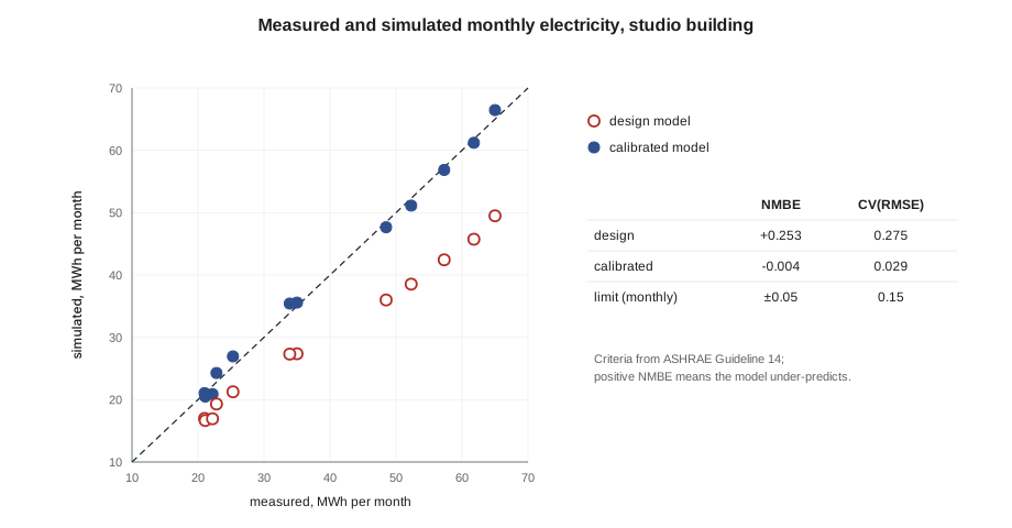
Calibrating the studio building

The students start with the simplest possible model of the studio building: monthly electricity equals the heat pumps' heating energy, proportional to the building's conductance and the month's heating degree-days, plus a constant base load for lights, plugs, fans and pumps. The design model used the conductance and base load from the renovation drawings. They compare it with the twelve monthly bills, then search for the pair of values that best fits.

# Calibrating an energy model of the studio building against twelve monthly meter readings
import math
HDD = [880, 720, 560, 290, 110, 20, 5, 8, 80, 280, 520, 790]   # heating degree-days by month, base 18 C (65 F); multiply by 1.8 for F-days
meter = [54.1, 47.6, 43.9, 30.5, 22.9, 20.2, 20.9, 21.7, 21.2, 29.8, 41.3, 52.5]                                   # metered electricity, MWh per month
days = [31, 28, 31, 30, 31, 30, 31, 31, 30, 31, 30, 31]
def model(ua_kw_per_k, plug_kw):
    """Monthly MWh: heat pump heating (seasonal COP 2.5) plus constant plug, light and fan load."""
    return [ua_kw_per_k * h * 24 / 2.5 / 1000 + plug_kw * d * 24 / 1000 for h, d in zip(HDD, days)]
def nmbe(m, s):
    n = len(m); return sum(a - b for a, b in zip(m, s)) / ((n - 1) * sum(m) / n)
def cvrmse(m, s):
    n = len(m); mean = sum(m) / n
    return math.sqrt(sum((a - b) ** 2 for a, b in zip(m, s)) / (n - 1)) / mean
first = model(3.0, 22.0)                              # values from the design drawings
print(f"design model:     NMBE {nmbe(meter, first):+.3f}  CV(RMSE) {cvrmse(meter, first):.3f}")
best = None; passing = 0
for ua10 in range(20, 61):                             # search conductance 2.0 to 6.0 kW/K
    for plug in range(10, 41):                         # and base load 10 to 40 kW
        s = model(ua10 / 10, plug)
        err = cvrmse(meter, s)
        if err <= 0.15 and abs(nmbe(meter, s)) <= 0.05:
            passing += 1
        if best is None or err < best[0]:
            best = (err, ua10 / 10, plug, s)
err, ua, plug, s = best
print(f"calibrated model: NMBE {nmbe(meter, s):+.3f}  CV(RMSE) {err:.3f}  conductance {ua:.1f} kW/K, base load {plug} kW")
print(f"pairs of values that also meet the monthly criteria: {passing} of {41 * 31}")
print("monthly criteria in ASHRAE Guideline 14: NMBE within 0.05, CV(RMSE) within 0.15")

design model:     NMBE +0.244  CV(RMSE) 0.262
calibrated model: NMBE -0.005  CV(RMSE) 0.034  conductance 4.2 kW/K, base load 27 kW
pairs of values that also meet the monthly criteria: 131 of 1271
monthly criteria in ASHRAE Guideline 14: NMBE within 0.05, CV(RMSE) within 0.15

The design model's NMBE of about +0.25 means it under-predicts by about a quarter, and its CV(RMSE) of about 0.27 is far outside the monthly limit of 0.15. A search over plausible values finds a calibrated model with a conductance of 4.2 kW/K instead of 3.0, and a base load of 27 kW instead of 22, which meets both criteria comfortably. The students now have explanations to investigate: is the envelope leakier than designed, or the ventilation running longer? Are there more computers, or a server room nobody mentioned?

The third line of output carries Holm's real lesson. About 131 of the 1,271 pairs of values the search tried also meet the monthly criteria. A higher conductance with a lower base load, or the reverse, fits the bills almost as well, because with monthly data the two effects are hard to separate: both raise winter use, and only the base load raises summer use, so the fit depends on a handful of summer months. This problem, that many different combinations of inputs reproduce the same measurements, is called equifinality. It means a calibrated model is not unique, and that meeting the criteria does not prove the inputs are right.

Better data, better calibration

Equifinality is reduced by more and better data. Hourly or fifteen-minute data separate night from day and weekday from weekend, which distinguishes envelope losses from occupancy-driven loads. Sub-meters on the heat pumps, the lighting panels and the plug circuits measure end uses directly. Short-term measurements, such as a blower door test, a week of logged temperatures in key rooms, or a spot measurement of ventilation flows, pin down individual inputs. Holm's team on a school project in Denmark found that a single blower door test and two weeks of logged ventilation flows cut the number of plausible model variants from hundreds to a handful.

With the right data, calibration becomes an investigation. Callum asks the facilities staff about the studio building's operation and learns that its ventilation runs around the clock because a timer failed two winters ago, and that the model shop's dust collector and kilns were added after the renovation. The ventilation fault explains most of the higher conductance; the new equipment explains most of the higher base load. The calibration found a fault that is costing the school money, a common and valuable outcome.

Bayesian calibration

Researchers increasingly treat calibration as a problem of inference under uncertainty. In Bayesian calibration, the analyst starts with prior distributions for the uncertain inputs, representing what is known before looking at the data, and uses the measured data to update them into posterior distributions, which describe the plausible values given the evidence. The result is not one calibrated model but a family of them, weighted by how well they fit, and predictions made with the family carry their uncertainty with them. Bayesian methods need many model runs and are usually done with surrogate models, the subject of Lesson 12, but their logic is useful even informally: a calibration should narrow uncertainty, not pretend to remove it.

Uncertainty in design-stage predictions

At the design stage there is nothing to calibrate against, yet owners and codes increasingly want predictions: an expected energy bill, a net-zero balance, a carbon budget. Holm teaches a practical approach, which the students will use in their simulation project.

• Identify the important uncertain inputs with a sensitivity analysis, as in Lesson 5.
• Assign each a plausible range or distribution from defensible sources.
• Propagate the uncertainty by running the model many times, with sampled inputs, or with a surrogate model.
• Report the result as a range, such as the median and the values below which 10 and 90 in 100 of the runs fall.
• State which inputs contribute most to the range and what could narrow it.

Reporting a range is uncomfortable at first: clients want one number. But a range tells them something a single number hides: how much margin the design needs. If the net-zero balance is positive in 9 of 10 plausible futures but negative in the tenth, the client can decide whether to add more panels, specify efficient equipment, or accept the risk.

Closing the loop: monitoring after occupancy

Performance-based design does not end at handover. The loop of Lesson 1 closes with measurement in use: commissioning that checks systems work as designed, monitoring that tracks energy and comfort over the first years, and post-occupancy evaluation that asks people how the building works for them. A model calibrated with the first year's data becomes a tool for the operators, who can compare each month's use with the model's prediction for the actual weather and spot faults early. Measurement and verification of this kind is required by some programs, such as ENERGY STAR benchmarking ordinances in Minneapolis and many other cities, which require large buildings to report their energy use each year, and it is the best way for designers to learn from their own buildings.

Exercise 11: calibrate a model

Each team of two calibrates a simple model of a campus building against a year of utility data.

• Collect the bills or interval data and the actual weather for the period.
• Run the design model with the actual weather and compare.
• Adjust only uncertain inputs, within plausible ranges, and record every change and its reason.
• Report NMBE and CV(RMSE) against the Guideline 14 criteria.
• Report how many input combinations meet the criteria, and what additional data would narrow them.

Self-critique checklist

• Did I use the actual weather of the measured period?
• Are my adjusted inputs physically plausible, and can I explain them?
• Have I acknowledged equifinality?
• Did I check my findings in the building with the people who run it?