Common discrete distributions

A handful of discrete distributions describe an enormous range of situations: the Bernoulli and binomial for successes in a fixed number of trials, the geometric and negative binomial for waiting times measured in trials, the hypergeometric for sampling without replacement, and the Poisson for counts of rare events in time or space. Each arises from a simple story, and knowing the story is the best way to know when the distribution applies. This lesson derives each pmf from its story, computes its mean and variance, proves the relationships between them, and finishes with the Poisson limit theorem, which explains why the Poisson distribution turns up so often in insurance, epidemiology and quality control.

Bernoulli and binomial

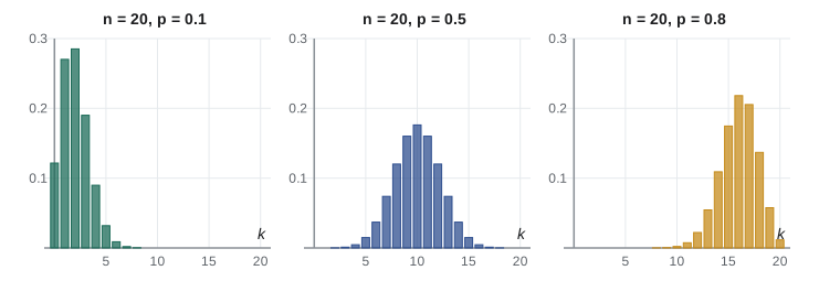
A Bernoulli trial has two outcomes, success with probability \(p\) and failure with probability \(1 - p\). The indicator of success, \(X \sim \text{Bernoulli}(p)\), has \(E[X] = p\) and \(\operatorname{Var}(X) = p - p^2 = p(1 - p)\). The binomial distribution counts successes in \(n\) independent Bernoulli trials with the same \(p\). A particular sequence with \(k\) successes has probability \(p^k(1 - p)^{n - k}\) by independence, and there are \(\binom{n}{k}\) such sequences, so

The probabilities sum to \((p + (1 - p))^n = 1\) by the binomial theorem, which is where the distribution gets its name. Writing \(X\) as a sum of \(n\) independent Bernoulli indicators gives the mean and variance immediately, with no algebra on the pmf: \(E[X] = np\) and \(\operatorname{Var}(X) = np(1 - p)\). The pmf rises while \(P(X = k + 1)/P(X = k) = \frac{(n - k)p}{(k + 1)(1 - p)} > 1\), so its mode is \(\lfloor (n + 1)p \rfloor\). The sum of independent binomials with the same \(p\) is binomial: \(\text{Bin}(m, p) + \text{Bin}(n, p) = \text{Bin}(m + n, p)\), since both count successes in a longer run of trials.

The assumptions matter. The trials must be independent and must share the same \(p\). The number of infected people in a household is not binomial, because infection spreads within households; the number of defectives in a day's production is not binomial if the defect rate drifts during the day. When the assumptions fail, the variance of the count is usually larger than \(np(1 - p)\), a phenomenon called overdispersion.

Geometric and negative binomial

Run independent Bernoulli trials until the first success. The number of trials \(X\) needed is geometric: \(P(X = k) = (1 - p)^{k - 1}p\) for \(k = 1, 2, \ldots\). Its survival function is \(P(X > k) = (1 - p)^k\), the chance that the first \(k\) trials all fail. Using the tail-sum formula of lesson 6, \(E[X] = \sum_{k \ge 0}(1 - p)^k = 1/p\): a die needs on average 6 rolls to show a six. The variance is \((1 - p)/p^2\). Some books count failures before the first success instead, \(Y = X - 1\), with mean \((1 - p)/p\); the weekly claims model of lesson 4 was of this form. The geometric distribution is memoryless, \(P(X > m + n \mid X > m) = P(X > n)\), and is the only memoryless distribution on the positive integers.

The negative binomial generalizes the geometric to the number of trials \(X\) needed for the \(r\)th success. The \(r\)th success happens on trial \(k\) when trial \(k\) is a success and exactly \(r - 1\) of the previous \(k - 1\) are, so

\(X\) is the sum of \(r\) independent geometric waiting times, so \(E[X] = r/p\) and \(\operatorname{Var}(X) = r(1 - p)/p^2\). Actuaries use the negative binomial for claim counts that are more variable than the Poisson allows, and epidemiologists use it for counts of secondary infections, where a few superspreaders cause most of the cases.

Hypergeometric

Draw \(n\) items without replacement from a population of \(N\) containing \(K\) successes. Lesson 2 showed that the number of successes \(X\) has

Write \(X\) as a sum of indicators \(I_1 + \cdots + I_n\), where \(I_j\) indicates that the \(j\)th draw is a success. By symmetry each draw is equally likely to be any item, so \(P(I_j = 1) = K/N\) and \(E[X] = nK/N\), the same as for sampling with replacement. The variance is smaller: with \(p = K/N\), \(\operatorname{Var}(X) = np(1 - p)\frac{N - n}{N - 1}\). The factor \((N - n)/(N - 1)\), the finite population correction, reflects the negative dependence between draws: drawing a success makes the next draw slightly less likely to be one. Lesson 9 derives it from covariances. When \(n\) is a small fraction of \(N\) the correction is close to 1 and the binomial is an excellent approximation.

Poisson

\(X\) is Poisson with mean \(\lambda > 0\) if

The probabilities sum to 1 because \(\sum \lambda^k/k! = e^\lambda\). For the mean, \(E[X] = \sum_{k \ge 1} k e^{-\lambda}\lambda^k/k! = \lambda\sum_{k \ge 1}e^{-\lambda}\lambda^{k-1}/(k-1)! = \lambda\). A similar shift computes \(E[X(X - 1)] = \lambda^2\), so \(E[X^2] = \lambda^2 + \lambda\) and \(\operatorname{Var}(X) = \lambda\). Mean equals variance is the Poisson signature, and comparing the two in data is the first check of whether a Poisson model is reasonable.

The sum of independent Poisson variables is Poisson: if \(X \sim \text{Poisson}(\lambda)\) and \(Y \sim \text{Poisson}(\mu)\) are independent, the convolution gives \(P(X + Y = n) = \sum_k e^{-\lambda}\frac{\lambda^k}{k!}e^{-\mu}\frac{\mu^{n-k}}{(n-k)!} = \frac{e^{-(\lambda + \mu)}}{n!}\sum_k\binom{n}{k}\lambda^k\mu^{n-k} = e^{-(\lambda+\mu)}\frac{(\lambda + \mu)^n}{n!}\). So claims from two independent regions, each Poisson, total to a Poisson count with the combined mean. Conversely, if each of a Poisson number of events is independently of type A with probability \(q\), the type A count is Poisson with mean \(\lambda q\) and independent of the type B count. This thinning property lets an insurer split a Poisson stream of claims into small and large ones and model each separately.

The Poisson limit theorem

Why is the Poisson so common? Because it is the limit of the binomial when there are many trials, each with a small chance of success. Let \(X_n \sim \text{Bin}(n, p_n)\) with \(np_n \to \lambda\). For fixed \(k\),

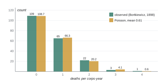
As \(n \to \infty\) the first factor tends to \(\lambda^k/k!\), the second to 1, the third to \(e^{-\lambda}\) because \((1 - \lambda/n)^n \to e^{-\lambda}\), and the fourth to 1. So \(P(X_n = k) \to e^{-\lambda}\lambda^k/k!\). The theorem explains why the number of claims on a large portfolio of independent policies, the number of typos on a page, the number of mutations in a stretch of DNA and the number of calls to a help line in a minute are all approximately Poisson: each is a count of many unlikely, roughly independent events. The classical example, analysed by Ladislaus Bortkiewicz in 1898, was the number of Prussian cavalry soldiers killed each year by horse kicks, which fit a Poisson distribution with mean about 0.61 remarkably well.

The approximation is good when \(n\) is large and \(p\) small; a rule of thumb is \(n \ge 20\) and \(p \le 0.05\). Le Cam's inequality makes it precise: the total variation distance between \(\text{Bin}(n, p)\) and \(\text{Poisson}(np)\) is at most \(np^2\), and the bound extends to sums of independent Bernoulli trials with different probabilities \(p_i\), where it becomes \(\sum p_i^2\). That generalization is what really justifies Poisson models for insurance portfolios whose policies have different risks.

from math import comb, exp, factorial
import random

def binom_pmf(k, n, p):  return comb(n, k) * p**k * (1 - p)**(n - k)
def pois_pmf(k, lam):     return exp(-lam) * lam**k / factorial(k)
def hyper_pmf(k, N, K, n): return comb(K, k) * comb(N - K, n - k) / comb(N, n)

print(" k   Bin(200000,2e-5)  Poisson(4)")
for k in range(0, 9):
    print(f"{k:2d}   {binom_pmf(k, 200_000, 2e-5):.6f}        {pois_pmf(k, 4):.6f}")
tv = 0.5 * sum(abs(binom_pmf(k, 200_000, 2e-5) - pois_pmf(k, 4)) for k in range(60))
print(f"total variation distance {tv:.2e}  (Le Cam bound {200_000 * 2e-5**2:.1e})")

# hypergeometric vs binomial: sample 10 from 60 items with 12 defective
for k in range(0, 5):
    print(f"k = {k}: hypergeometric {hyper_pmf(k, 60, 12, 10):.4f}  binomial {binom_pmf(k, 10, 0.2):.4f}")

# Poisson signature: simulated mean and variance; thinning
rng = random.Random(251)
def poisson(lam):              # count unit-rate exponential arrivals before time lam
    t, k = 0.0, -1
    while t <= lam:
        t += rng.expovariate(1.0); k += 1
    return k
xs = [poisson(4) for _ in range(100_000)]
m = sum(xs) / len(xs); v = sum((x - m) ** 2 for x in xs) / len(xs)
large = [sum(rng.random() < 0.25 for _ in range(x)) for x in xs[:50_000]]
ml = sum(large) / len(large)
print(f"Poisson(4) sample mean {m:.3f}, variance {v:.3f}; thinned mean {ml:.3f} (expected 1.000)")

 k   Bin(200000,2e-5)  Poisson(4)
 0   0.018315        0.018316
 1   0.073261        0.073263
 2   0.146524        0.146525
 3   0.195368        0.195367
 4   0.195369        0.195367
 5   0.156295        0.156293
 6   0.104196        0.104196
 7   0.059540        0.059540
 8   0.029770        0.029770
total variation distance 5.01e-06  (Le Cam bound 8.0e-05)
k = 0: hypergeometric 0.0868  binomial 0.1074
k = 1: hypergeometric 0.2669  binomial 0.2684
k = 2: hypergeometric 0.3303  binomial 0.3020
k = 3: hypergeometric 0.2148  binomial 0.2013
k = 4: hypergeometric 0.0806  binomial 0.0881
Poisson(4) sample mean 3.994, variance 3.998; thinned mean 0.999 (expected 1.000)

Choosing a discrete model

The stories decide the model. A fixed number of independent trials with the same success probability gives the binomial. Waiting for the first or \(r\)th success gives the geometric or negative binomial. Sampling without replacement from a finite population gives the hypergeometric. Counting rare events in a period of time or a region of space, when events occur independently at a steady rate, gives the Poisson. Data can then check the choice. If counts have variance much larger than their mean, a Poisson model understates risk, and an insurer that priced on it would set aside too little for bad years; the negative binomial, which arises as a Poisson whose mean is itself random, is the usual remedy.

A historical data set: deaths from horse kicks

The horse-kick data mentioned above come from Ladislaus von Bortkiewicz's book Das Gesetz der kleinen Zahlen (The Law of Small Numbers), published in 1898. He recorded the number of soldiers killed by horse kicks in 10 Prussian cavalry corps over 20 years, from 1875 to 1894, giving 200 corps-years. In 109 corps-years there were no deaths, in 65 one death, in 22 two, in 3 three and in 1 four. The total is \(65 + 44 + 9 + 4 = 122\) deaths, so the average is \(\hat{\lambda} = 122/200 = 0.61\) per corps-year.

If deaths in a corps-year are Poisson with mean 0.61, the expected number of corps-years with \(k\) deaths is \(200e^{-0.61}0.61^k/k!\). Since \(e^{-0.61} \approx 0.5434\), this gives about 108.7, 66.3, 20.2, 4.1 and 0.6 for \(k = 0, 1, 2, 3, 4\). The agreement with the observed counts is striking, and the reason is the Poisson limit theorem: each soldier had a tiny, roughly independent chance of a fatal kick in a year, and there were many soldiers. The sample variance of the counts is also close to the mean, as the Poisson model requires: \(\frac{1}{200}(65 + 88 + 27 + 16) - 0.61^2 = 0.98 - 0.3721 = 0.6079\). A variance well above the mean (overdispersion) would suggest that the rate differs between corps or years, and a model such as the negative binomial would fit better.

The same reasoning applies to modern counts of rare events spread over many independent opportunities: misprints per page, goals per hockey game, calls per minute to a help line, and mutations per generation. When counts are much more variable than the Poisson model allows, the clustering itself is informative; insurance claims after a storm, for example, arrive together rather than independently.