Functions of random variables and moment generating functions

Once we know the distribution of \(X\), we often need the distribution of something computed from it: the area \(\pi R^2\) of a disc whose radius is random, the log of a stock price, the total of several independent claims, the maximum of a set of flood levels. This lesson collects the standard tools. The cdf method works almost always. The change-of-variable formula is a shortcut for smooth one-to-one transformations. Convolution handles sums of independent variables, and moment generating functions turn sums into products, which makes them the most efficient way to identify the distribution of a sum. The same tools prove the inverse transform method that every simulation library relies on, and they set up the proof of the central limit theorem in the next lesson.

The cdf method

To find the distribution of \(Y = g(X)\), compute its cdf directly: \(F_Y(y) = P(g(X) \le y)\), rewrite the event in terms of \(X\), and differentiate to get the density. Take \(X\) uniform on \((0, 1)\) and \(Y = -\ln X\). For \(y > 0\), \(P(Y \le y) = P(\ln X \ge -y) = P(X \ge e^{-y}) = 1 - e^{-y}\), so \(Y\) is exponential with rate 1. For a non-monotone example, take \(Z\) standard normal and \(Y = Z^2\). For \(y > 0\), \(F_Y(y) = P(-\sqrt{y} \le Z \le \sqrt{y}) = \Phi(\sqrt{y}) - \Phi(-\sqrt{y})\). Differentiating with the chain rule gives \(f_Y(y) = \frac{1}{\sqrt{y}}\varphi(\sqrt{y}) = \frac{1}{\sqrt{2\pi y}}e^{-y/2}\), the chi-squared distribution with one degree of freedom, which is the gamma distribution with shape \(1/2\) and rate \(1/2\). This is the starting point of the chi-squared tests used throughout statistics.

The cdf method also handles maxima and minima of independent variables, which matter in reliability and hydrology. If \(X_1, \dots, X_n\) are independent with cdf \(F\), then \(M = \max X_i\) satisfies \(P(M \le m) = P(\text{all } X_i \le m) = F(m)^n\). The minimum satisfies \(P(\min X_i > m) = (1 - F(m))^n\). For independent exponential lifetimes with rates \(\lambda_1, \dots, \lambda_n\), \(P(\min > t) = e^{-(\lambda_1 + \cdots + \lambda_n)t}\): the first failure is exponential with the summed rate. A system of components in series fails at the first failure, so its failure rate is the sum of the component failure rates.

The change-of-variable formula

If \(g\) is strictly increasing and differentiable with inverse \(h\), then \(F_Y(y) = P(X \le h(y)) = F_X(h(y))\), and differentiating gives \(f_Y(y) = f_X(h(y))h'(y)\). If \(g\) is strictly decreasing, \(F_Y(y) = 1 - F_X(h(y))\) and the derivative picks up a minus sign, which cancels the negative \(h'\). The two cases combine into one formula:

The factor \(|h'(y)|\) is the stretching factor: an interval of length \(dy\) near \(y\) corresponds to an interval of length \(|h'(y)|\,dy\) near \(x = h(y)\), and probability is conserved. For a linear transformation \(Y = aX + b\) with \(a \ne 0\), \(f_Y(y) = \frac{1}{|a|}f_X\big(\frac{y - b}{a}\big)\). This shows at once that a linear function of a normal variable is normal, with mean \(a\mu + b\) and standard deviation \(|a|\sigma\).

The lognormal is the standard model for stock prices and for many sizes in nature (incomes, particle sizes, insurance losses) because it arises from multiplying many independent positive factors: the log of a product is a sum, and sums tend to be normal. The fact that the mean exceeds \(e^\mu\) matters in finance: if annual log returns average 5% with a standard deviation of 20%, the expected growth factor is \(e^{0.05 + 0.02} \approx 1.0725\), not \(e^{0.05} \approx 1.0513\), while the median growth factor is \(e^{0.05}\).

Why inverse transform sampling works

Lesson 5 used the inverse transform method to simulate from a cdf \(F\). Here is the proof. Suppose \(F\) is continuous and strictly increasing, and let \(U\) be uniform on \((0, 1)\). Set \(X = F^{-1}(U)\). Then \(P(X \le x) = P(F^{-1}(U) \le x) = P(U \le F(x)) = F(x)\), because \(F\) is increasing and \(P(U \le u) = u\). So \(X\) has cdf \(F\). The converse, called the probability integral transform, also holds: if \(X\) has continuous cdf \(F\), then \(F(X)\) is uniform on \((0, 1)\), since \(P(F(X) \le u) = P(X \le F^{-1}(u)) = u\). For a general cdf, which may have jumps and flat parts, the same argument works with the generalized inverse \(F^{-1}(u) = \min\{x : F(x) \ge u\}\). This is exactly how a discrete distribution is sampled: draw \(U\) and return the first value at which the cumulative probability reaches \(U\).

Two-dimensional transformations

For a smooth one-to-one map from \((X_1, X_2)\) to \((Y_1, Y_2)\), the joint density transforms with the absolute value of the Jacobian determinant of the inverse map: \(f_Y(y_1, y_2) = f_X(x_1, x_2)\,|J|\), where \(J = \det\big(\partial(x_1, x_2)/\partial(y_1, y_2)\big)\). This is the two-dimensional version of the stretching factor. The classic application is polar coordinates. If \(X\) and \(Y\) are independent standard normals, their joint density is \(\frac{1}{2\pi}e^{-(x^2 + y^2)/2}\). In polar coordinates \(x = r\cos\theta\), \(y = r\sin\theta\), with Jacobian \(r\), the density becomes \(\frac{1}{2\pi}\cdot re^{-r^2/2}\) on \(r > 0\), \(0 < \theta < 2\pi\). It factors, so the angle is uniform and independent of the radius, and \(R^2\) is exponential with mean 2. Reversing this gives the Box–Muller method (1958): from two independent uniforms, set \(R = \sqrt{-2\ln U_1}\) and \(\Theta = 2\pi U_2\), and \(R\cos\Theta\), \(R\sin\Theta\) are independent standard normals. The same calculation evaluates \(\int e^{-x^2/2}dx = \sqrt{2\pi}\), the normalizing constant of the normal density.

Sums of independent variables: convolution

If \(X\) and \(Y\) are independent and \(S = X + Y\), then in the discrete case \(P(S = s) = \sum_x P(X = x)P(Y = s - x)\), and in the continuous case

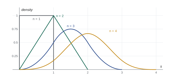
This operation is called convolution. For two independent uniforms on \((0, 1)\), the integrand is 1 when \(0 < x < 1\) and \(0 < s - x < 1\), so \(f_S(s) = s\) for \(0 \le s \le 1\) and \(2 - s\) for \(1 \le s \le 2\): a triangle. Adding a third uniform gives a piecewise quadratic that already looks bell-shaped. For two independent exponentials with rate \(\lambda\), \(f_S(s) = \int_0^s \lambda e^{-\lambda x}\lambda e^{-\lambda(s - x)}\,dx = \lambda^2 se^{-\lambda s}\), the gamma density with shape 2, which is the waiting time to the second event of a Poisson process. Convolution integrals quickly get messy, which is why the next tool is so useful.

Moment generating functions

The moment generating function (MGF) of \(X\) is \(M_X(t) = E[e^{tX}]\), defined for the values of \(t\) where the expectation is finite. Three properties make it useful.

• Moments: expanding \(e^{tX} = \sum_k t^kX^k/k!\) and taking expectations gives \(M_X(t) = \sum_k E[X^k]t^k/k!\), so \(E[X^k] = M_X^{(k)}(0)\). The MGF packages all the moments, hence the name.

• Sums: if \(X\) and \(Y\) are independent, \(M_{X+Y}(t) = E[e^{tX}e^{tY}] = M_X(t)M_Y(t)\). Convolution of densities becomes multiplication of MGFs. Linear changes are simple too: \(M_{aX + b}(t) = e^{bt}M_X(at)\).

• Uniqueness: if two random variables have MGFs that are finite and equal on an open interval around 0, they have the same distribution. So identifying an MGF identifies a distribution.

The standard MGFs follow from the definitions. Bernoulli: \(1 - p + pe^t\). Binomial: \((1 - p + pe^t)^n\), the product of \(n\) Bernoulli MGFs. Poisson: \(\sum_k e^{tk}e^{-\lambda}\lambda^k/k! = e^{\lambda(e^t - 1)}\). Exponential with rate \(\lambda\): \(\int_0^\infty e^{tx}\lambda e^{-\lambda x}\,dx = \frac{\lambda}{\lambda - t}\) for \(t < \lambda\). Gamma with shape \(\alpha\) and rate \(\lambda\): \(\big(\frac{\lambda}{\lambda - t}\big)^\alpha\). Normal: completing the square, as in the lognormal example, gives

Identifying sums with MGFs

The product rule and uniqueness together settle the distribution of many sums at once.

• Independent Poisson(\(\lambda_1\)) and Poisson(\(\lambda_2\)): \(e^{\lambda_1(e^t - 1)}e^{\lambda_2(e^t - 1)} = e^{(\lambda_1 + \lambda_2)(e^t - 1)}\), so the sum is Poisson(\(\lambda_1 + \lambda_2\)). Calls to two independent help lines merge into one Poisson stream.

• Independent normals \(N(\mu_1, \sigma_1^2)\) and \(N(\mu_2, \sigma_2^2)\): the product of MGFs is \(e^{(\mu_1 + \mu_2)t + (\sigma_1^2 + \sigma_2^2)t^2/2}\), so the sum is \(N(\mu_1 + \mu_2, \sigma_1^2 + \sigma_2^2)\). Means add and variances add; standard deviations do not.

• \(n\) independent exponentials with rate \(\lambda\): \(\big(\frac{\lambda}{\lambda - t}\big)^n\), the gamma with shape \(n\), confirming the convolution result without integrals.

• Independent binomials with the same \(p\): \(\text{Bin}(m, p) + \text{Bin}(n, p) = \text{Bin}(m + n, p)\). With different \(p\) the product is not of binomial form, and the sum is not binomial.

A caution about MGFs: they need not exist. The Cauchy distribution and heavy-tailed distributions such as the Pareto have \(E[e^{tX}] = \infty\) for every \(t > 0\), and the lognormal has finite moments of every order but no MGF. Probabilists then use the characteristic function \(E[e^{itX}]\), which always exists because \(|e^{itX}| = 1\), and which has the same product and uniqueness properties. The generating function idea goes back to de Moivre and Laplace in the eighteenth century; Laplace used it systematically in his Théorie analytique des probabilités (1812).

import random, math
from fractions import Fraction
from statistics import mean, pvariance

rng = random.Random(251)
N = 200_000

# cdf method: -ln U is exponential(1); Z^2 is chi-squared(1) with mean 1, variance 2
e = [-math.log(1 - rng.random()) for _ in range(N)]
z2 = [rng.gauss(0, 1) ** 2 for _ in range(N)]
print(f"-ln U:  mean {mean(e):.3f} (1), var {pvariance(e):.3f} (1)")
print(f"Z^2:    mean {mean(z2):.3f} (1), var {pvariance(z2):.3f} (2)")

# lognormal mean: E[e^X] = exp(mu + s^2/2)
mu, s = 0.05, 0.20
print(f"E[exp(X)] ~ {mean(math.exp(rng.gauss(mu, s)) for _ in range(N)):.4f}  exact {math.exp(mu + s * s / 2):.4f}")

# Box-Muller
bm = random.Random(1958)
def box_muller():
    r = math.sqrt(-2 * math.log(1 - bm.random())); th = 2 * math.pi * bm.random()
    return r * math.cos(th), r * math.sin(th)
pts = [box_muller() for _ in range(N // 2)]
xs = [a for a, b in pts] + [b for a, b in pts]
print(f"Box-Muller: mean {mean(xs):.3f}, var {pvariance(xs):.3f}, P(|Z|<1.96) {sum(abs(x) < 1.96 for x in xs) / len(xs):.4f}")

# exact discrete convolution: total of three dice, with Fractions
die = {k: Fraction(1, 6) for k in range(1, 7)}
def convolve(p, q):
    r = {}
    for a, pa in p.items():
        for b, qb in q.items():
            r[a + b] = r.get(a + b, 0) + pa * qb
    return r
three = convolve(convolve(die, die), die)
print("P(total of three dice = 10) =", three[10], " P(= 9) =", three[9])

# moments from an MGF by finite differences: Poisson(3), M(t) = exp(3(e^t - 1))
M = lambda t: math.exp(3 * (math.exp(t) - 1)); h = 1e-4
m1 = (M(h) - M(-h)) / (2 * h); m2 = (M(h) - 2 * M(0) + M(-h)) / h ** 2
print(f"Poisson(3) from its MGF: mean {m1:.4f}, variance {m2 - m1 ** 2:.4f}")

# sum of two independent Poissons is Poisson
def poisson(lam):
    k, p, u = 0, math.exp(-lam), rng.random(); c = p
    while u > c:
        k += 1; p *= lam / k; c += p
    return k
s5 = [poisson(2) + poisson(3) for _ in range(N)]
print(f"P(sum = 5) simulated {s5.count(5) / N:.4f}, Poisson(5) value {math.exp(-5) * 5 ** 5 / 120:.4f}")

-ln U:  mean 1.003 (1), var 1.008 (1)
Z^2:    mean 1.002 (1), var 2.014 (2)
E[exp(X)] ~ 1.0720  exact 1.0725
Box-Muller: mean 0.000, var 0.995, P(|Z|<1.96) 0.9505
P(total of three dice = 10) = 1/8  P(= 9) = 25/216
Poisson(3) from its MGF: mean 3.0000, variance 3.0000
P(sum = 5) simulated 0.1755, Poisson(5) value 0.1755