Conditional probability, independence and Bayes' theorem

Probabilities change when we learn something. The chance that a patient has a disease is one number before a test and another after a positive result; the chance of rain tomorrow is one number in general and another given that a low-pressure system is moving in. Conditional probability is the rule for updating, and it is the most important idea in this course after the axioms themselves. From it come the multiplication rule for building probabilities in stages, the law of total probability for splitting a hard problem into easy cases, Bayes' theorem for reversing the direction of a conditional, and the notion of independence, which makes most of the models in the rest of the course possible.

Definition

If \(P(B) > 0\), the conditional probability of \(A\) given \(B\) is

The idea is that learning \(B\) occurred shrinks the sample space to \(B\). Outcomes outside \(B\) are ruled out, and outcomes inside \(B\) keep their relative probabilities, so they are rescaled to add up to 1. With equally likely outcomes this becomes \(|A \cap B| / |B|\): count the outcomes in \(B\) that are also in \(A\). Roll two dice and learn that the total is 8. Of the 36 ordered outcomes, five give 8: (2,6), (3,5), (4,4), (5,3), (6,2). Given that, the probability of a double is 1/5, not the unconditional 1/6.

For a fixed \(B\) with \(P(B) > 0\), the function \(A \mapsto P(A \mid B)\) is itself a probability measure: it is non-negative, gives \(B\) (and so \(\Omega\)) probability 1, and is countably additive because intersecting disjoint events with \(B\) keeps them disjoint. Every theorem of lesson 1 therefore holds for conditional probabilities. In particular \(P(A^c \mid B) = 1 - P(A \mid B)\). Note that \(P(A \mid B)\) and \(P(A \mid B^c)\) need not add to 1; they are conditional on different events.

The multiplication rule

Rearranging the definition gives \(P(A \cap B) = P(B)P(A \mid B) = P(A)P(B \mid A)\). By induction, for any events with \(P(A_1 \cap \cdots \cap A_{n-1}) > 0\),

This is how we usually compute probabilities of sequences: one stage at a time, each conditional on what has already happened. The probability that the first three cards dealt are all aces is \(\frac{4}{52}\cdot\frac{3}{51}\cdot\frac{2}{50} = \frac{1}{5525}\). The acceptance-sampling calculation of lesson 2 was an application of the same rule.

The law of total probability

A partition of \(\Omega\) is a collection of disjoint events \(B_1, B_2, \ldots\) whose union is \(\Omega\): exactly one of them occurs. For any event \(A\),

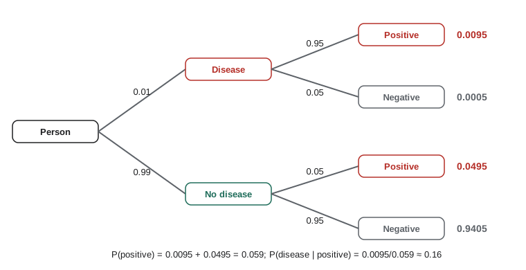
Proof: \(A\) is the disjoint union of the sets \(A \cap B_i\); apply countable additivity and the multiplication rule to each piece. The law lets us compute a probability by conditioning on whatever we wish we knew. An insurer whose drivers are 20% high risk, with a 15% chance of a claim in a year, and 80% low risk, with a 5% chance, sees claims from \(0.15 \times 0.2 + 0.05 \times 0.8 = 0.07\) of its drivers. Probability trees are pictures of exactly this calculation: branch on the partition, multiply along each path and add the paths that end in \(A\).

Bayes' theorem

Often we know \(P(A \mid B)\) but want \(P(B \mid A)\). A test's maker reports how often the test is positive in people who have the disease; a patient wants to know how likely the disease is given a positive result. Combining the definition with the law of total probability gives Bayes' theorem: for a partition \(B_1, B_2, \ldots\) and an event \(A\) with \(P(A) > 0\),

The terms have names. \(P(B_j)\) is the prior probability of \(B_j\), before \(A\) is observed. \(P(A \mid B_j)\) is the likelihood of the observation under \(B_j\). \(P(B_j \mid A)\) is the posterior probability. The theorem is named for the Reverend Thomas Bayes, whose essay on the subject was published in 1763, two years after his death; Laplace independently developed and used it much more widely.

The result surprises almost everyone, including many physicians in published surveys. The error of reading \(P(D \mid +)\) as if it were \(P(+ \mid D)\) is called the base-rate fallacy, or in legal settings the prosecutor's fallacy: the probability of the evidence given innocence is not the probability of innocence given the evidence. A clean way to see the right answer is to imagine 10,000 people. About 100 have the disease and 95 of them test positive; of the 9,900 without it, about 495 test positive. Of the 590 positives, only 95 are real.

Odds form of Bayes' theorem

For two hypotheses, Bayes' theorem is neatest in terms of odds. Dividing the formula for \(P(D \mid +)\) by the one for \(P(D^c \mid +)\) cancels the denominator:

Posterior odds are prior odds times the likelihood ratio. For the screening test the likelihood ratio is \(0.95/0.05 = 19\) and the prior odds are \(1/99\), so the posterior odds are \(19/99\), a probability of \(19/118 \approx 0.161\) as before. Each further independent positive multiplies the odds by 19 again. The odds form shows why a strong test can still give a weak conclusion: a likelihood ratio of 19 cannot overcome prior odds of 1 to 99 in a single step.

Independence

Events \(A\) and \(B\) are independent if \(P(A \cap B) = P(A)P(B)\). When \(P(B) > 0\) this is equivalent to \(P(A \mid B) = P(A)\): learning that \(B\) occurred does not change the probability of \(A\). The product form is preferred as the definition because it is symmetric and makes sense even when a probability is zero. If \(A\) and \(B\) are independent, so are \(A\) and \(B^c\): \(P(A \cap B^c) = P(A) - P(A \cap B) = P(A)(1 - P(B)) = P(A)P(B^c)\).

Independence of more than two events needs care. Events \(A_1, \ldots, A_n\) are mutually independent if for every subcollection \(A_{i_1}, \ldots, A_{i_k}\), the probability of the intersection is the product of the probabilities. Pairwise independence is weaker. Toss two fair coins and let \(A\) be 'first toss heads', \(B\) 'second toss heads' and \(C\) 'the tosses agree'. Each pair is independent, each with intersection probability 1/4, but \(P(A \cap B \cap C) = 1/4 \ne 1/8\): knowing \(A\) and \(B\) determines \(C\).

Independence is usually an assumption about the physical world, not something we prove: separate tosses of a coin, separate patients in a trial, separate components built in separate plants. It is what lets us multiply. A system of 10 components in series, each working with probability 0.99 independently, works with probability \(0.99^{10} \approx 0.904\). The same components in parallel, where the system works if any one does, fail together with probability \(0.01^{10}\). Wrongly assuming independence can be catastrophic: components sharing a power supply, mortgages sharing a housing market or patients sharing a hospital ward fail together far more often than the product rule predicts.

Conditional independence

Events \(A\) and \(B\) are conditionally independent given \(C\) if \(P(A \cap B \mid C) = P(A \mid C)P(B \mid C)\). Two screening tests may be conditionally independent given disease status, which is what we assumed when we updated twice. They are not unconditionally independent: a positive first test raises the chance of disease, which raises the chance of a positive second test. Conditional independence without unconditional independence is common, and confusing the two is a classic source of error.

import random
from fractions import Fraction

def posterior(prior, sens, spec, positives=1):
    p = Fraction(prior)
    for _ in range(positives):
        num = Fraction(sens) * p
        p = num / (num + (1 - Fraction(spec)) * (1 - p))
    return p

for prev in ("1/1000", "1/100", "1/10"):
    p1 = posterior(prev, "95/100", "95/100", 1)
    p2 = posterior(prev, "95/100", "95/100", 2)
    print(f"prevalence {prev:>6}: P(D|+) = {float(p1):.3f}, P(D|++) = {float(p2):.3f}")

# simulate 200,000 people with prevalence 1%
rng = random.Random(251)
n, pos, true_pos = 200_000, 0, 0
for _ in range(n):
    d = rng.random() < 0.01
    t = rng.random() < (0.95 if d else 0.05)
    if t:
        pos += 1
        true_pos += d
print(f"simulated P(D|+) = {true_pos / pos:.3f} from {pos} positives")

# pairwise but not mutually independent events: two fair coins
from itertools import product
om = list(product("HT", repeat=2))
P = lambda ev: Fraction(sum(1 for w in om if ev(w)), 4)
A = lambda w: w[0] == "H"; B = lambda w: w[1] == "H"; C = lambda w: w[0] == w[1]
print("P(A&B) =", P(lambda w: A(w) and B(w)), " P(A&C) =", P(lambda w: A(w) and C(w)),
      " P(A&B&C) =", P(lambda w: A(w) and B(w) and C(w)))

prevalence 1/1000: P(D|+) = 0.019, P(D|++) = 0.265
prevalence  1/100: P(D|+) = 0.161, P(D|++) = 0.785
prevalence   1/10: P(D|+) = 0.679, P(D|++) = 0.976
simulated P(D|+) = 0.160 from 11805 positives
P(A&B) = 1/4  P(A&C) = 1/4  P(A&B&C) = 1/4

The output makes the role of the prior concrete. At a prevalence of 1 in 1,000, a single positive leaves the probability of disease below 2%. At 1 in 10, as in a clinic for people with symptoms, the same test gives about 68%. The test has not changed; the population has. This is why guidelines distinguish screening the general population from testing people with symptoms.

The Monty Hall problem

A game show has three doors, one hiding a car. You pick door 1. The host, who knows where the car is and always opens a losing door you did not pick, opens door 3 to show a goat and offers to let you switch to door 2. Should you? Let \(C_i\) be 'car behind door \(i\)', each with prior 1/3, and \(H_3\) 'host opens door 3'. Then \(P(H_3 \mid C_1) = 1/2\), since the host chooses at random between doors 2 and 3; \(P(H_3 \mid C_2) = 1\); and \(P(H_3 \mid C_3) = 0\). Bayes gives \(P(C_2 \mid H_3) = 1 \cdot \tfrac13 / (\tfrac12 \cdot \tfrac13 + 1 \cdot \tfrac13 + 0) = 2/3\). Switching wins two times in three. The answer depends on the host's rule: if he opened a door at random and happened to reveal a goat, the two remaining doors would be equally likely. Probability depends on how information is obtained, not just on what is observed.

Bayes' theorem with repeated tests

Positive screening results are usually followed by a second, independent test. Bayes' theorem can be applied twice: the posterior after the first test becomes the prior for the second. In the screening example with prevalence 1%, sensitivity 95% and false positive rate 5%, a first positive result raises the probability of disease to about 0.161. A second independent positive result gives \(\frac{0.161 \times 0.95}{0.161 \times 0.95 + 0.839 \times 0.05} \approx 0.785\). The odds form makes this quick: each positive result multiplies the odds by the likelihood ratio \(0.95/0.05 = 19\), so the prior odds of \(1/99\) become \(19/99\) and then \(361/99\), a probability of \(361/460 \approx 0.785\). The calculation assumes the two results are conditionally independent given disease status, which fails if both tests react to the same harmless condition.