Continuous random variables and densities

Lifetimes, rainfall amounts, response times, heights and measurement errors can take any value in an interval, not just values from a list. For such quantities the probability of any single exact value is zero, and a pmf is useless. Probability is instead spread smoothly along the line, like mass along a wire, and described by a density. This lesson defines continuous random variables and their densities, relates densities to cdfs through the fundamental theorem of calculus, works through the uniform and exponential families, and introduces the memoryless property and the hazard rate, the two ideas reliability engineers and actuaries use most.

Densities

A random variable \(X\) is continuous if there is a function \(f \ge 0\), its probability density function or pdf, such that for every interval

Taking the interval to be the whole line shows that \(\int_{-\infty}^{\infty} f(x)\,dx = 1\). Conversely, any non-negative integrable function with total integral 1 is the density of some random variable. Probability is area under the density curve. Two consequences follow at once. First, \(P(X = a) = \int_a^a f = 0\) for every \(a\), so for continuous variables it does not matter whether interval endpoints are included: \(P(a < X < b) = P(a \le X \le b)\). Second, a density value is not a probability and can exceed 1. The uniform density on \([0, 0.5]\) is 2 everywhere on the interval.

What a density value does measure is probability per unit length. For a small \(h\), \(P(x \le X \le x + h) \approx f(x)h\) when \(f\) is continuous at \(x\). A density of 0.3 per hour at \(t = 10\) hours means that the chance of failure between 10 hours and 10 hours and 1 minute is about \(0.3/60 = 0.005\). This is why densities change when the units change: if \(X\) is measured in minutes instead of hours, its density is divided by 60.

Density and cdf

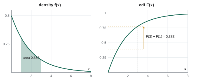
The cdf of a continuous variable is \(F(x) = P(X \le x) = \int_{-\infty}^{x} f(t)\,dt\). It is continuous everywhere, since there are no jumps, and by the fundamental theorem of calculus \(F'(x) = f(x)\) at every point where \(f\) is continuous. So the density is the derivative of the cdf, and the cdf is the integral of the density. In practice we often find one from the other. Interval probabilities come straight from the cdf: \(P(a < X \le b) = F(b) - F(a)\).

Not every random variable is discrete or continuous. An insurance claim might be zero with probability 0.9 (no claim filed) and otherwise follow a density on the positive amounts. Its cdf jumps at 0 and then rises smoothly. Such mixed distributions are common in actuarial work and in data with a detection limit, and the cdf handles them without fuss: it is the one description that works for every random variable.

The uniform distribution

\(X\) is uniform on \([a, b]\) if its density is constant there: \(f(x) = 1/(b - a)\) for \(a \le x \le b\) and 0 elsewhere. Its cdf rises linearly from 0 at \(a\) to 1 at \(b\): \(F(x) = (x - a)/(b - a)\). The probability of any subinterval is its length divided by \(b - a\). The uniform distribution on \((0, 1)\) plays a special role, because computers generate it (approximately) and every other distribution can be built from it by the inverse transform of lesson 4. A rounding error, the arrival time of a bus that comes every 15 minutes at a random moment, and the phase of a wave are natural uniform variables.

The exponential distribution

\(X\) is exponential with rate \(\lambda > 0\) if \(f(x) = \lambda e^{-\lambda x}\) for \(x \ge 0\) and 0 for \(x < 0\). Integrating, \(F(x) = 1 - e^{-\lambda x}\) and the survival function is \(S(x) = P(X > x) = e^{-\lambda x}\). The exponential is the standard model for the waiting time until an event that happens at a constant rate: the time to the next radioactive decay, the time between calls at a help line, the time to failure of an electronic component with no wear. Lesson 6 shows that its mean is \(1/\lambda\), so a component failing at rate 0.002 per hour has a mean life of 500 hours.

The exponential distribution is memoryless: for all \(s, t \ge 0\),

A component that has survived \(s\) hours is, as far as its future is concerned, as good as new. That is exactly right for some things, such as radioactive atoms and fuses that fail only from random surges, and badly wrong for others, such as bearings, tires and people, which wear out. A deeper fact is that the exponential is the only continuous distribution with this property. If \(S\) is a survival function with \(S(s + t) = S(s)S(t)\) for all \(s, t \ge 0\), then \(g = \log S\) satisfies \(g(s + t) = g(s) + g(t)\); a monotone solution of this equation is linear, \(g(t) = -\lambda t\), so \(S(t) = e^{-\lambda t}\). Its discrete counterpart, the geometric distribution, is likewise the only memoryless distribution on the positive integers.

Hazard rates

For a lifetime \(T\) with density \(f\) and survival function \(S\), the hazard rate is

the instantaneous failure rate of items that have survived to time \(t\). The exponential has constant hazard \(\lambda\), which is another way of saying it is memoryless. A hazard that increases with age describes wear-out; one that decreases describes infant mortality, where weak items fail early and the survivors are the strong ones. Many products show both, giving the bathtub-shaped hazard of reliability engineering. Since \(h(t) = -\frac{d}{dt}\log S(t)\), the hazard determines the distribution: \(S(t) = \exp(-H(t))\), where \(H(t) = \int_0^t h(u)\,du\) is the cumulative hazard. Lesson 8 meets the Weibull family, whose hazard \(h(t) = k\lambda^k t^{k-1}\) increases, decreases or stays constant as \(k\) is above, below or equal to 1.

Normalizing constants and support

Densities are often given up to a constant, which is then found by integrating. If \(f(x) = cx^2\) on \([0, 3]\), then \(1 = c\int_0^3 x^2\,dx = 9c\), so \(c = 1/9\). The set where the density is positive is called the support. Always state it. The formula \(f(x) = cx^2\) means nothing until we say where it applies, and many errors in integration come from integrating a density beyond its support. For densities on unbounded supports, check that the integral converges: \(f(x) = c/x^2\) on \([1, \infty)\) works with \(c = 1\), but \(f(x) = c/x\) on \([1, \infty)\) cannot be normalized for any \(c\), because \(\int_1^\infty dx/x\) diverges.

Numerical integration

Many densities, including the normal, have no elementary antiderivative, so their probabilities are computed numerically. Simpson's rule, which fits parabolas through pairs of subintervals, is accurate enough for nearly every practical purpose and is easy to write. The code below normalizes \(f(x) = cx^2\) on \([0, 3]\), computes probabilities for the exponential pump model both exactly and with Simpson's rule, and checks the memoryless property by simulation.

import math, random

def simpson(f, a, b, n=1000):          # n must be even
    h = (b - a) / n
    s = f(a) + f(b) + sum((4 if i % 2 else 2) * f(a + i * h) for i in range(1, n))
    return s * h / 3

c = 1 / simpson(lambda x: x * x, 0, 3)
print(f"normalizing constant for c x^2 on [0, 3]: {c:.6f} (exact 1/9 = {1/9:.6f})")

lam = 0.25
f = lambda t: lam * math.exp(-lam * t)
print(f"P(T <= 2): Simpson {simpson(f, 0, 2):.6f}, exact {1 - math.exp(-0.5):.6f}")
print(f"total mass up to 80 years: {simpson(f, 0, 80):.6f}")

rng = random.Random(251)
T = [rng.expovariate(lam) for _ in range(200_000)]
alive4 = [t for t in T if t > 4]
p_cond = sum(t > 6 for t in alive4) / len(alive4)
p_new = sum(t > 2 for t in T) / len(T)
print(f"P(T > 6 | T > 4) simulated {p_cond:.4f};  P(T > 2) simulated {p_new:.4f}")
print(f"sample median {sorted(T)[len(T) // 2]:.3f}  vs  4 ln 2 = {4 * math.log(2):.3f}")

normalizing constant for c x^2 on [0, 3]: 0.111111 (exact 1/9 = 0.111111)
P(T <= 2): Simpson 0.393469, exact 0.393469
total mass up to 80 years: 1.000000
P(T > 6 | T > 4) simulated 0.6083;  P(T > 2) simulated 0.6069
sample median 2.785  vs  4 ln 2 = 2.773

Simpson's rule with 1,000 subintervals reproduces the exact answers to six decimals. The simulated conditional probability of surviving 2 more years among pumps that reached 4 years matches the unconditional probability of reaching 2 years, as memorylessness predicts, and the sample median lands near \(4\ln 2\). For a distribution with wear-out, such as a Weibull with \(k = 2\), the same simulation would show old pumps doing worse than new ones.

Percentiles in practice

Engineering and environmental standards are often written in terms of percentiles of continuous distributions. A rainfall that is exceeded with probability 0.01 in any year is called the 100-year rainfall, and drainage is designed to carry it; a structural load exceeded with probability 0.05 over the design life is a characteristic load. For a continuous cdf the \(q\) quantile solves \(F(x_q) = q\) exactly. For the exponential, \(x_q = -\ln(1 - q)/\lambda\). For the pump, the 90th percentile of lifetime is \(-\ln(0.1)/0.25 \approx 9.2\) years: one pump in ten lasts longer than that. The 100-year event, despite its name, has probability \(1 - 0.99^{30} \approx 0.26\) of occurring at least once in a 30-year mortgage, which is a fact many homeowners in flood-prone areas do not know.

Worked example: waiting at a bus stop

The result can be surprising: both routes average one bus every 10 minutes, yet the random route doubles the expected wait. The explanation is the inspection paradox. A rider arriving at a random time is more likely to land in a long gap between buses than a short one, because long gaps cover more of the clock. With exponential gaps of mean 10, the gap containing a random arrival has mean 20 minutes, and the rider waits on average half of it. Transit agencies in Canadian cities track headway regularity for exactly this reason: bunching of buses raises the average wait even when the number of buses per hour is unchanged.

The same paradox appears in many surveys. Asking people currently in hospital how long their stay is overstates the typical stay, because long stays are more likely to be in progress on any given day. Asking students about the size of their classes overstates the average class size, because large classes contain more students to ask.