The law of large numbers and the central limit theorem

Two theorems explain why probability works in practice. The law of large numbers says that the average of many independent repetitions settles down to the expected value, which is why a casino, an insurer and a pollster can rely on long-run averages even though each individual outcome is unpredictable. The central limit theorem says more: the fluctuations of the average around its expected value are approximately normal, whatever the distribution of the individual terms, with a size that shrinks like \(1/\sqrt{n}\). Together they justify confidence intervals, margins of error, quality control charts and most of statistical inference. This lesson proves the weak law from Chebyshev's inequality, states the central limit theorem and sketches its proof with moment generating functions, and puts both to work with the normal approximation to the binomial and the continuity correction.

The sample mean

Let \(X_1, X_2, \dots\) be independent and identically distributed (i.i.d.) with mean \(\mu\) and variance \(\sigma^2\), and let \(\bar{X}_n = (X_1 + \cdots + X_n)/n\). By linearity \(E[\bar{X}_n] = \mu\), and because variances of independent terms add, \(\operatorname{Var}(\bar{X}_n) = n\sigma^2/n^2 = \sigma^2/n\). The standard deviation of the average, \(\sigma/\sqrt{n}\), is called the standard error. These two lines contain the core of everything that follows: the average is centred on the right value, and its spread shrinks with \(\sqrt{n}\). Quadrupling the sample halves the standard error, which is why polls of 1,000 and 4,000 people differ in precision by a factor of two, not four.

Markov's and Chebyshev's inequalities

Two inequalities bound tail probabilities using only a mean or a variance. Markov's inequality: if \(X \ge 0\) and \(a > 0\), then \(P(X \ge a) \le E[X]/a\). Proof: \(X \ge a\mathbf{1}\{X \ge a\}\) pointwise, and taking expectations gives \(E[X] \ge aP(X \ge a)\). Applying Markov to the non-negative variable \((X - \mu)^2\) with \(a = k^2\) gives Chebyshev's inequality:

Chebyshev's inequality holds for every distribution with a finite variance, so it is often crude: it says that at most 25% of any distribution lies two or more standard deviations from the mean, where the normal value is about 4.6%. Its value lies in its generality. The inequality is named after Pafnuty Chebyshev, who published it in 1867; Irénée-Jules Bienaymé had stated it earlier, in 1853, and it is sometimes called the Bienaymé–Chebyshev inequality.

The weak law of large numbers

Apply Chebyshev to \(\bar{X}_n\), which has mean \(\mu\) and variance \(\sigma^2/n\). For any \(\varepsilon > 0\),

This is the weak law of large numbers: the sample mean converges in probability to \(\mu\). The first version, for Bernoulli trials, is due to Jacob Bernoulli, whose Ars Conjectandi was published posthumously in 1713. His proof was much longer, because the variance tools above did not yet exist. The strong law of large numbers, proved in full generality by Kolmogorov in the 1930s, says more: with probability 1, the sequence \(\bar{X}_n\) actually converges to \(\mu\). The weak law says that for each large \(n\), a big deviation is unlikely; the strong law says that, along almost every infinite sequence of outcomes, the deviations eventually stay small forever. Both need only a finite mean for i.i.d. sequences, though our proof used a finite variance.

The law of large numbers is often misread as a force that corrects past deviations. It is not. After ten heads in a row, a fair coin is still fair; the proportion of heads returns towards one half because the initial excess of ten is swamped by thousands of later tosses, not because tails become more likely. The belief that a run of heads makes tails due is the gambler's fallacy. In 1913, at the Monte Carlo casino, black came up 26 times in a row at roulette, and gamblers lost heavily betting on red.

The central limit theorem

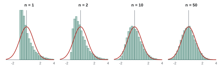
The law of large numbers tells us that \(\bar{X}_n - \mu \to 0\). The central limit theorem (CLT) tells us the shape of the deviation when it is magnified by \(\sqrt{n}\). With i.i.d. terms of mean \(\mu\) and finite variance \(\sigma^2 > 0\), let \(S_n = X_1 + \cdots + X_n\). Then for every real \(z\),

In words: a sum of many independent, identically distributed terms is approximately normal with mean \(n\mu\) and variance \(n\sigma^2\), and the average is approximately \(N(\mu, \sigma^2/n)\). The remarkable part is that the shape of the terms does not matter. They can be dice, coin tosses, exponential waiting times or claim sizes. Only the mean and variance survive in the limit. This is why the normal distribution appears whenever a quantity is the accumulated effect of many small, roughly independent influences, from measurement errors to heights.

A sketch of the proof

The MGF method gives a short proof when the MGF of the terms exists near 0. Standardize: let \(Y_i = (X_i - \mu)/\sigma\), which have mean 0 and variance 1, and let \(Z_n = (Y_1 + \cdots + Y_n)/\sqrt{n}\). By independence and the scaling rule,

Expand \(M_Y\) near 0 using its moments: \(M_Y(s) = 1 + E[Y]s + E[Y^2]s^2/2 + o(s^2) = 1 + s^2/2 + o(s^2)\). With \(s = t/\sqrt{n}\), \(M_{Z_n}(t) = \big(1 + \frac{t^2}{2n} + o(1/n)\big)^n \to e^{t^2/2}\), using the limit \((1 + a/n + o(1/n))^n \to e^a\). The limit is the MGF of the standard normal. A continuity theorem (if MGFs converge on an interval around 0, the cdfs converge at every point) completes the argument. The general proof, which needs only a finite variance, is the same argument with characteristic functions, which always exist. Look at where the hypotheses were used: the mean zero killed the linear term, the variance one fixed the quadratic term, and the higher moments disappeared in the limit. That is why only \(\mu\) and \(\sigma^2\) survive.

History

Abraham de Moivre found the first case in 1733, for the binomial distribution with \(p = 1/2\), while approximating sums of binomial coefficients; he used what is now called Stirling's formula and obtained the normal curve as the limit. He included the result in the second edition of The Doctrine of Chances (1738). Pierre-Simon Laplace extended it to general \(p\) and to sums of other variables, in work culminating in his Théorie analytique des probabilités (1812), so the binomial case is now called the de Moivre–Laplace theorem. A rigorous proof under general conditions was given by Aleksandr Lyapunov in 1901, and Jarl Lindeberg in 1922 and Paul Lévy found the conditions now taught. The name central limit theorem was coined by George Pólya in 1920, central in the sense of being of central importance.

The normal approximation to the binomial

A Binomial(\(n, p\)) count is a sum of \(n\) independent Bernoulli(\(p\)) terms, so for large \(n\) it is approximately \(N(np, np(1 - p))\). A common rule of thumb asks for \(np \ge 10\) and \(n(1 - p) \ge 10\); the approximation is poor for very skewed binomials, where the Poisson approximation is better. Because the binomial takes integer values and the normal is continuous, the approximation improves with the continuity correction: treat the integer \(k\) as the interval \([k - 0.5, k + 0.5]\). So \(P(X \le k) \approx \Phi\big(\frac{k + 0.5 - np}{\sqrt{np(1-p)}}\big)\) and \(P(X \ge k) \approx 1 - \Phi\big(\frac{k - 0.5 - np}{\sqrt{np(1-p)}}\big)\).

Sums with the CLT

The CLT applies to any sum of many independent terms, not just counts. Suppose an insurer's 10,000 home policies have independent annual losses with a mean of 650 dollars and a standard deviation of 4,000 dollars (most policies claim nothing, a few claim a lot). The total loss has mean 6.5 million dollars and standard deviation \(4000\sqrt{10000} = 400{,}000\). The probability that total losses exceed 7.3 million, two standard deviations above the mean, is about \(1 - \Phi(2) \approx 0.023\). The relative variability of the total, \(400{,}000/6{,}500{,}000 \approx 6\%\), is far smaller than that of a single policy, whose standard deviation is six times its mean. This is the law of large numbers and the CLT at work in the business of insurance. The calculation assumes independence; a single hailstorm over Calgary, which can cause over a billion dollars of insured damage, violates it, which is why insurers buy reinsurance.

When the CLT fails or is slow

The theorem needs a finite variance. The Cauchy distribution, the ratio of two independent standard normals, has no mean at all, and the average of \(n\) Cauchy variables has exactly the same Cauchy distribution as a single one: averaging does not help. Heavy-tailed data such as earthquake energies, city sizes and some financial losses can behave similarly. Even with a finite variance, the approximation can be slow for skewed terms. The Berry–Esseen theorem quantifies this: the maximum error in the cdf is at most \(C\rho/(\sigma^3\sqrt{n})\), where \(\rho = E|X - \mu|^3\) and \(C\) is a constant below 0.48. So skewness slows convergence, and the error shrinks like \(1/\sqrt{n}\). Dependence also matters: positively correlated terms make the sum more variable than \(\sigma\sqrt{n}\) suggests.

import random, math
from statistics import mean, pstdev, NormalDist

rng = random.Random(251)
Phi = NormalDist().cdf

# law of large numbers: running proportion of sixes
sixes, checkpoints = 0, {10, 100, 1000, 10_000, 100_000}
for n in range(1, 100_001):
    sixes += rng.randint(1, 6) == 6
    if n in checkpoints:
        print(f"n = {n:>6}: proportion of sixes {sixes / n:.4f}  (1/6 = {1/6:.4f})")

# CLT: standardized mean of n exponential(1) variables
for n in (1, 2, 10, 50):
    zs = [(mean(rng.expovariate(1) for _ in range(n)) - 1) * math.sqrt(n) for _ in range(20_000)]
    print(f"n = {n:>2}: P(Z <= -1) = {sum(z <= -1 for z in zs) / len(zs):.4f}, "
          f"P(Z > 1.645) = {sum(z > 1.645 for z in zs) / len(zs):.4f}  (normal: 0.1587, 0.0500)")

# overbooking: exact binomial against the normal approximation
n, p = 200, 0.92
exact = sum(math.comb(n, k) * p ** k * (1 - p) ** (n - k) for k in range(191, n + 1))
mu, sd = n * p, math.sqrt(n * p * (1 - p))
print(f"P(X >= 191): exact {exact:.4f}, with continuity correction {1 - Phi((190.5 - mu) / sd):.4f}, "
      f"without {1 - Phi((191 - mu) / sd):.4f}")

# Chebyshev against the truth for a normal variable
for k in (1.5, 2, 3):
    print(f"k = {k}: Chebyshev bound {1 / k ** 2:.3f}, normal value {2 * (1 - Phi(k)):.4f}")

# the Cauchy distribution: averaging does not help
for n in (1, 100, 10_000):
    means = [mean(rng.gauss(0, 1) / rng.gauss(0, 1) for _ in range(n)) for _ in range(200)]
    print(f"Cauchy, n = {n:>5}: share of means with |mean| > 3 = {sum(abs(m) > 3 for m in means) / 200:.3f}")

n =     10: proportion of sixes 0.3000  (1/6 = 0.1667)
n =    100: proportion of sixes 0.1500  (1/6 = 0.1667)
n =   1000: proportion of sixes 0.1690  (1/6 = 0.1667)
n =  10000: proportion of sixes 0.1672  (1/6 = 0.1667)
n = 100000: proportion of sixes 0.1663  (1/6 = 0.1667)
n =  1: P(Z <= -1) = 0.0000, P(Z > 1.645) = 0.0729  (normal: 0.1587, 0.0500)
n =  2: P(Z <= -1) = 0.1159, P(Z > 1.645) = 0.0724  (normal: 0.1587, 0.0500)
n = 10: P(Z <= -1) = 0.1562, P(Z > 1.645) = 0.0631  (normal: 0.1587, 0.0500)
n = 50: P(Z <= -1) = 0.1546, P(Z > 1.645) = 0.0554  (normal: 0.1587, 0.0500)
P(X >= 191): exact 0.0374, with continuity correction 0.0451, without 0.0340
k = 1.5: Chebyshev bound 0.444, normal value 0.1336
k = 2: Chebyshev bound 0.250, normal value 0.0455
k = 3: Chebyshev bound 0.111, normal value 0.0027
Cauchy, n =     1: share of means with |mean| > 3 = 0.180
Cauchy, n =   100: share of means with |mean| > 3 = 0.190
Cauchy, n = 10000: share of means with |mean| > 3 = 0.155