Sample spaces, events and the axioms of probability

Probability is the mathematics of uncertainty. It tells an insurer how much to set aside for claims it cannot predict one by one, tells an epidemiologist how likely an outbreak is to fade out on its own, tells an engineer how often a bridge component will see a load above its rating, and tells a statistician how far an estimate computed from a sample is likely to be from the truth. STAT-141 and STAT-151 used probability as a tool, mostly through tables, software and the normal curve. This course builds the subject itself. We start from three axioms and derive, with proofs, everything else: conditional probability and Bayes' theorem, random variables and their distributions, expectation and variance, joint distributions, transformations, generating functions, the law of large numbers and the central limit theorem. STAT-252 then uses these results to build the theory of estimation and testing.

The course uses calculus throughout. Densities are integrated, sums are manipulated as series, and limits appear whenever we let the number of trials grow. You will also write proofs. Most are short, but each one is there because it shows why a result is true, which is what lets you recognize when it applies and when it does not. Every lesson includes runnable Python that simulates the experiments we analyse, so you can compare an exact answer with what happens when the experiment is carried out thousands of times. When the two agree, you gain confidence in both; when they disagree, one of them is wrong, and finding out which is one of the best ways to learn.

A short history

The modern subject began with a correspondence in 1654 between Blaise Pascal and Pierre de Fermat about the problem of points: how should the stakes be divided when a game of chance is interrupted before it is finished? Their answer, which counts the ways the game could have continued, is still the standard one. Over the next two centuries Jacob Bernoulli proved the first law of large numbers, Abraham de Moivre found the normal approximation to the binomial distribution, and Pierre-Simon Laplace wrote a great treatise that applied probability to astronomy, demography and the reliability of testimony. What the subject lacked was a foundation. Probability was defined in different ways for different problems, and paradoxes appeared when the definitions were stretched.

In 1933 Andrey Kolmogorov supplied the foundation in a short book that put probability on the same footing as the rest of mathematics. He defined a probability as a function on a collection of sets satisfying three axioms, borrowing the ideas of measure theory developed by Lebesgue and others. Everything in this course rests on Kolmogorov's axioms. What the axioms do not tell you is what a probability means. Some people read a probability as a long-run relative frequency, others as a degree of belief; both readings obey the same axioms, and both are used in practice. We will mostly use the frequency reading, because it is the one simulation makes concrete.

Experiments and sample spaces

A random experiment is any process whose outcome is not known in advance: rolling a die, testing a patient, recording tomorrow's rainfall, counting the claims an insurer receives in a week. The sample space \(\Omega\) is the set of all possible outcomes. Choosing it is the first modelling decision and sometimes the most important one.

• Toss a coin three times. \(\Omega = \{HHH, HHT, HTH, HTT, THH, THT, TTH, TTT\}\), with 8 outcomes.

• Count the claims in a week. \(\Omega = \{0, 1, 2, \ldots\}\), which is countably infinite.

• Measure the lifetime of a pump in hours. \(\Omega = [0, \infty)\), which is uncountable.

• Pick a point at random in a unit square. \(\Omega = [0, 1]^2\).

The same physical experiment can be described by different sample spaces. For three coin tosses we could instead record only the number of heads, \(\Omega' = \{0, 1, 2, 3\}\). The coarser space loses information: from \(\Omega'\) we cannot ask whether the first toss was heads. A good rule is to choose a sample space fine enough to describe every question you might want to ask, and in which the outcomes are easy to assign probabilities to. For coins and dice that usually means outcomes that are equally likely.

Events and the algebra of sets

An event is a subset of the sample space: a collection of outcomes. We say the event \(A\) occurs when the outcome of the experiment lies in \(A\). For three tosses, the event 'at least two heads' is \(A = \{HHH, HHT, HTH, THH\}\). The whole space \(\Omega\) is the certain event and the empty set \(\varnothing\) is the impossible event.

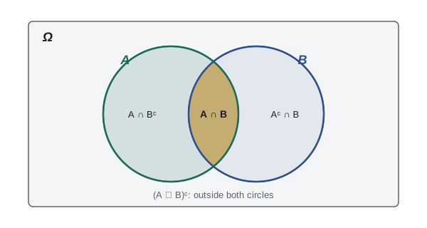
Logical combinations of events are set operations. The union \(A \cup B\) is the event that \(A\) or \(B\) (or both) occurs; the intersection \(A \cap B\) is the event that both occur; the complement \(A^c = \Omega \setminus A\) is the event that \(A\) does not occur; and the difference \(A \setminus B = A \cap B^c\) is the event that \(A\) occurs but \(B\) does not. Two events are disjoint, or mutually exclusive, if \(A \cap B = \varnothing\): they cannot both occur.

Two identities, De Morgan's laws, are used constantly:

In words, 'not (A or B)' is 'not A and not B', and 'not (A and B)' is 'not A or not B'. Both extend to any number of events, including infinitely many. To prove the first, take an outcome \(\omega\). It lies in \((A \cup B)^c\) exactly when it is in neither \(A\) nor \(B\), which is exactly when it lies in \(A^c\) and in \(B^c\). Two sets with the same elements are equal, so the identity holds.

Kolmogorov's axioms

A probability measure assigns to each event \(A\) a number \(P(A)\). Kolmogorov required three things:

• Axiom 1 (non-negativity): \(P(A) \ge 0\) for every event \(A\).

• Axiom 2 (normalization): \(P(\Omega) = 1\).

• Axiom 3 (countable additivity): if \(A_1, A_2, \ldots\) are pairwise disjoint events, then \(P(A_1 \cup A_2 \cup \cdots) = \sum_{i=1}^{\infty} P(A_i)\).

The third axiom is the one with content. It says that probability behaves like area or mass: the probability of a region made of non-overlapping pieces is the sum of the probabilities of the pieces. Requiring this for infinitely many pieces, not just finitely many, is what makes limits work later in the course. For an uncountable sample space such as \([0, 1]\) there is a technical subtlety: it is impossible to assign a probability to every subset of \([0, 1]\) in a way that satisfies the axioms and gives each interval its length. The fix is to restrict attention to a large collection of well-behaved subsets, called a sigma-algebra, which contains every set you will ever meet in practice. We note the subtlety once and then, as almost every applied text does, ignore it.

Consequences of the axioms

Everything else about probability is a theorem. The following properties follow from the axioms with short proofs, and they are worth proving once so that you never have to wonder whether they are true.

Theorem 1. \(P(\varnothing) = 0\). Proof: the sets \(\Omega, \varnothing, \varnothing, \ldots\) are pairwise disjoint and their union is \(\Omega\). Countable additivity gives \(P(\Omega) = P(\Omega) + \sum P(\varnothing)\). The sum of infinitely many copies of a non-negative number is finite only if the number is 0.

Theorem 2 (finite additivity). If \(A_1, \ldots, A_n\) are pairwise disjoint, \(P(A_1 \cup \cdots \cup A_n) = P(A_1) + \cdots + P(A_n)\). Proof: extend the list with \(A_{n+1} = A_{n+2} = \cdots = \varnothing\) and apply Axiom 3 and Theorem 1.

Theorem 3 (complements). \(P(A^c) = 1 - P(A)\). Proof: \(A\) and \(A^c\) are disjoint with union \(\Omega\), so \(P(A) + P(A^c) = 1\).

Theorem 4 (monotonicity). If \(A \subseteq B\) then \(P(A) \le P(B)\). Proof: \(B\) is the disjoint union of \(A\) and \(B \setminus A\), so \(P(B) = P(A) + P(B \setminus A) \ge P(A)\). In particular \(P(A) \le P(\Omega) = 1\) for every event.

Theorem 5 (inclusion–exclusion for two events). \(P(A \cup B) = P(A) + P(B) - P(A \cap B)\). Proof: write \(A \cup B\) as the disjoint union of \(A\) and \(B \setminus A\), and \(B\) as the disjoint union of \(A \cap B\) and \(B \setminus A\). Then \(P(A \cup B) = P(A) + P(B \setminus A)\) and \(P(B) = P(A \cap B) + P(B \setminus A)\). Subtract to eliminate \(P(B \setminus A)\).

For three events the formula becomes

and in general you add the single probabilities, subtract the pairwise intersections, add the triple intersections and so on with alternating signs. The idea behind the signs is that each outcome in the union must be counted exactly once. An outcome lying in exactly \(k\) of the events is counted \(\binom{k}{1} - \binom{k}{2} + \binom{k}{3} - \cdots = 1\) times, by the binomial theorem applied to \((1 - 1)^k = 0\).

Theorem 6 (Boole's inequality, or the union bound). For any events, \(P(A_1 \cup A_2 \cup \cdots) \le \sum P(A_i)\). Proof: define \(B_1 = A_1\) and \(B_i = A_i \setminus (A_1 \cup \cdots \cup A_{i-1})\). The \(B_i\) are disjoint, have the same union as the \(A_i\), and satisfy \(B_i \subseteq A_i\). Apply Axiom 3 and monotonicity. The union bound is crude but extremely useful: if each of 20 safety checks fails with probability at most 0.001, the chance that at least one fails is at most 0.02, whatever the dependence between them.

Continuity of probability

Countable additivity has a consequence that justifies many limit arguments. If the events increase, \(A_1 \subseteq A_2 \subseteq \cdots\), with union \(A\), then \(P(A_n) \to P(A)\). To prove it, write \(A\) as the disjoint union of \(A_1, A_2 \setminus A_1, A_3 \setminus A_2, \ldots\). By Axiom 3, \(P(A)\) is the sum of their probabilities, and the partial sums of that series are exactly \(P(A_n)\). By taking complements, the same holds for decreasing events: if \(B_1 \supseteq B_2 \supseteq \cdots\) with intersection \(B\), then \(P(B_n) \to P(B)\).

Here is a use. Let \(B_n\) be the event that the first \(n\) tosses of a fair coin are all heads, so \(P(B_n) = 2^{-n}\). The events decrease, and their intersection is the event that every toss is heads forever. By continuity its probability is \(\lim 2^{-n} = 0\). That event is not impossible, since the outcome HHH... is in the sample space, but it has probability zero. Probability zero and impossible are different things once the sample space is infinite, a point that will matter again for continuous random variables, where every single value has probability zero.

Equally likely outcomes

When \(\Omega\) is finite and every outcome is equally likely, the axioms force \(P(\{\omega\}) = 1/|\Omega|\) for each outcome, and therefore

This is the classical definition of probability used by Pascal and Fermat, now a consequence of the axioms rather than a definition. It turns probability problems into counting problems, which is the subject of lesson 2. Be careful: the formula needs the outcomes to be equally likely, and choosing a sample space in which they are is part of the work. The number of heads in three tosses takes the values 0, 1, 2, 3, but these are not equally likely; the eight sequences are.

Simulation as a check

The frequency reading of probability says that if an experiment is repeated many times independently, the fraction of trials in which \(A\) occurs settles down to \(P(A)\). Lesson 11 proves this as the law of large numbers. For now we use it as a working tool. The program below simulates the classical problem of the duke of Tuscany, who noticed that a total of 10 seemed to come up more often than a total of 9 when three dice were thrown, even though each total can be made in six ways. Galileo explained the puzzle by counting ordered outcomes. The code counts them exactly and compares the exact answer with a simulation of 200,000 throws.

import random
from itertools import product
from fractions import Fraction

outcomes = list(product(range(1, 7), repeat=3))     # 216 ordered outcomes
def exact(total):
    return Fraction(sum(1 for o in outcomes if sum(o) == total), len(outcomes))

rng = random.Random(251)
n = 200_000
counts = {9: 0, 10: 0}
for _ in range(n):
    s = rng.randint(1, 6) + rng.randint(1, 6) + rng.randint(1, 6)
    if s in counts:
        counts[s] += 1

for t in (9, 10):
    p = exact(t)
    print(f"total {t}: exact {p} = {float(p):.5f}, simulated {counts[t] / n:.5f}")
# unordered patterns that make each total: both have six
pat = lambda t: sorted({tuple(sorted(o)) for o in outcomes if sum(o) == t})
print("patterns for 9: ", pat(9))
print("patterns for 10:", pat(10))

total 9: exact 25/216 = 0.11574, simulated 0.11535
total 10: exact 1/8 = 0.12500, simulated 0.12502
patterns for 9:  [(1, 2, 6), (1, 3, 5), (1, 4, 4), (2, 2, 5), (2, 3, 4), (3, 3, 3)]
patterns for 10: [(1, 3, 6), (1, 4, 5), (2, 2, 6), (2, 3, 5), (2, 4, 4), (3, 3, 4)]

Both totals have six unordered patterns, but the patterns are not equally likely. The pattern \(3, 3, 3\) can occur in only one order, the pattern \(1, 2, 6\) in six orders. Counting the 216 ordered outcomes, which are equally likely, gives 25 ways to make 9 and 27 ways to make 10. The simulation agrees to two or three decimal places, which is about what we should expect from 200,000 trials; lesson 11 makes that precise. The lesson of the example is the one stated above: the classical formula is only as good as the sample space you apply it to.

Probability as a model

A probability model is a sample space together with a probability measure on its events. The axioms do not tell you which model to use; that is a modelling choice, justified by symmetry, by data or by judgement. A model for claim counts might say that the number of claims in a week is 0 with probability 0.30, 1 with probability 0.36, 2 with probability 0.22 and so on. Any assignment of non-negative numbers to the outcomes that sums to 1 defines a valid model on a countable sample space, because Axiom 3 then determines the probability of every event as a sum. Whether the model fits the insurer's experience is a statistical question, which STAT-252 addresses.

Throughout the course we will meet a small number of models over and over: the binomial for counts of successes, the Poisson for counts of rare events, the exponential for waiting times, the normal for measurements that are sums of many small effects. Part of the skill of probability is recognizing which model a situation calls for, and part is knowing what follows from that choice.