Expectation, variance and moments

A distribution is a whole function, but we often want a few numbers that summarize it: where it is centred, how spread out it is, how lopsided. The expected value, or mean, is the probability-weighted average of the values a random variable can take. It is the number an insurer charges as the pure premium, the long-run average payout of a lottery ticket, the centre of mass of the distribution. Variance measures spread around the mean, and higher moments describe shape. This lesson defines these quantities for discrete and continuous variables, proves the properties that make them so useful, above all the linearity of expectation, and shows two classic inequalities that bound probabilities using only a mean and a variance.

Expected value

For a discrete random variable with pmf \(p\), and a continuous one with density \(f\), the expected value is

provided the sum or integral converges absolutely, that is \(\sum |x|p(x) < \infty\) or \(\int |x|f(x)\,dx < \infty\). If it does not, the expectation does not exist. Physically, \(E[X]\) is the balance point of the distribution: if the pmf were made of weights on a rod, the rod would balance at \(E[X]\). It need not be a possible value. The expected number of heads in one toss of a fair coin is 1/2, and the expected face of a die is 3.5.

Two first examples. If \(X\) is exponential with rate \(\lambda\), integration by parts gives \(E[X] = \int_0^\infty x\lambda e^{-\lambda x}\,dx = [-xe^{-\lambda x}]_0^\infty + \int_0^\infty e^{-\lambda x}\,dx = 1/\lambda\). If \(X\) is uniform on \([a, b]\), symmetry gives \(E[X] = (a + b)/2\). Both should match intuition: an event at rate 2 per hour takes on average half an hour to happen, and the centre of an interval is its midpoint.

Not every distribution has a mean. The Cauchy density \(f(x) = 1/(\pi(1 + x^2))\) from lesson 5 is symmetric about 0, but \(\int |x|/(\pi(1 + x^2))\,dx\) diverges like \(\int dx/x\). Its tails are so heavy that sample averages never settle down: the average of a million Cauchy observations has exactly the same distribution as a single one. Heavy-tailed losses in insurance and finance can behave similarly, which is why actuaries worry about whether the moments they estimate exist at all.

The law of the unconscious statistician

To find the expectation of \(g(X)\), we do not need the distribution of \(g(X)\). For discrete \(X\), \(E[g(X)] = \sum_x g(x)p(x)\), and for continuous \(X\), \(E[g(X)] = \int g(x)f(x)\,dx\). The discrete proof groups terms: \(E[g(X)] = \sum_y y\,P(g(X) = y) = \sum_y y\sum_{x : g(x) = y} p(x) = \sum_x g(x)p(x)\). The name, which is a joke about how often students use the result without noticing it needs proof, is standard. With it, \(E[X^2]\) for a fair die is \((1 + 4 + 9 + 16 + 25 + 36)/6 = 91/6\).

Linearity

Expectation is linear: for any random variables \(X\) and \(Y\) whose expectations exist and any constants \(a\), \(b\),

For discrete variables on a countable sample space, the proof is a rearrangement: \(E[X] = \sum_\omega X(\omega)P(\{\omega\})\), so \(E[aX + bY] = \sum_\omega (aX(\omega) + bY(\omega))P(\{\omega\}) = aE[X] + bE[Y]\), the rearrangement being justified by absolute convergence. The general case follows from the definition of the integral. The striking thing is what the theorem does not require: \(X\) and \(Y\) need not be independent. Linearity holds for any dependence whatsoever.

Combined with indicators, linearity is one of the most powerful tools in probability, because \(E[I_A] = P(A)\). To find the expected value of a count, write the count as a sum of indicators and add their probabilities. The expected number of heads in \(n\) tosses with heads probability \(p\) is \(np\). The expected number of letters that reach their own envelope in the matching problem of lesson 2 is \(n \times (1/n) = 1\), for every \(n\), even though the distribution of that number took inclusion–exclusion to find. The expected number of pairs sharing a birthday among \(n\) people is \(\binom{n}{2}/365\), which is about 0.69 for 23 people.

Expectation of products and independence

If \(X\) and \(Y\) are independent, then \(E[XY] = E[X]E[Y]\). For discrete variables, \(E[XY] = \sum_{x,y} xy\,P(X = x)P(Y = y) = (\sum_x xP(X = x))(\sum_y yP(Y = y))\). Without independence this fails in general. If \(X\) is \(\pm1\) with equal probability and \(Y = X\), then \(E[XY] = E[X^2] = 1\) while \(E[X]E[Y] = 0\). Unlike linearity, the product rule needs independence, or at least zero covariance, as lesson 9 explains.

Variance and standard deviation

The variance of \(X\) is the expected squared distance from the mean, \(\operatorname{Var}(X) = E[(X - \mu)^2]\) with \(\mu = E[X]\). Expanding the square and using linearity gives the computing formula

The standard deviation \(\sigma = \sqrt{\operatorname{Var}(X)}\) is in the same units as \(X\). For a fair die, \(\operatorname{Var}(X) = 91/6 - (7/2)^2 = 35/12 \approx 2.92\), so \(\sigma \approx 1.71\). For the exponential, \(E[X^2] = 2/\lambda^2\) by integrating by parts twice, so \(\operatorname{Var}(X) = 1/\lambda^2\) and the standard deviation equals the mean. For the uniform on \([a, b]\), \(\operatorname{Var}(X) = (b - a)^2/12\).

Variance has three key properties. It is never negative, and it is zero only if \(X\) equals its mean with probability 1. Shifting does not change it and scaling multiplies it by the square: \(\operatorname{Var}(aX + b) = a^2\operatorname{Var}(X)\). And for independent variables variances add, \(\operatorname{Var}(X + Y) = \operatorname{Var}(X) + \operatorname{Var}(Y)\). The last follows from expanding \(E[(X - \mu_X + Y - \mu_Y)^2]\): the cross term is \(2E[(X - \mu_X)(Y - \mu_Y)]\), which is \(2E[X - \mu_X]E[Y - \mu_Y] = 0\) under independence. Standard deviations do not add. The standard deviation of a sum of \(n\) independent copies of \(X\) is \(\sigma\sqrt{n}\), not \(n\sigma\), which is the root of every result about averages in this course.

Moments and shape

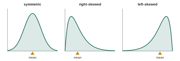
The \(k\)th moment of \(X\) is \(E[X^k]\) and the \(k\)th central moment is \(E[(X - \mu)^k]\). The mean is the first moment and the variance the second central moment. The third and fourth central moments, scaled by the standard deviation, describe shape. Skewness \(E[(X - \mu)^3]/\sigma^3\) is zero for symmetric distributions, positive for a long right tail, as with claim sizes and incomes, and negative for a long left tail. Kurtosis \(E[(X - \mu)^4]/\sigma^4\) measures the weight of the tails relative to the normal distribution, whose kurtosis is 3. The exponential has skewness 2 and kurtosis 9. Moments are not always finite, and a distribution can have a finite mean and an infinite variance; the Pareto distributions used for large insurance losses are the standard examples.

Markov's and Chebyshev's inequalities

Means and variances bound probabilities even when the distribution is unknown. Markov's inequality says that for a non-negative random variable \(X\) and any \(a > 0\),

Proof: \(X \ge aI_{\{X \ge a\}}\), because the right side is \(a\) when \(X \ge a\) and 0 otherwise; take expectations. If the average claim is 2,000 dollars, at most 10% of claims can exceed 20,000 dollars, whatever the distribution. Applying Markov to \((X - \mu)^2\) and \(a = k^2\sigma^2\) gives Chebyshev's inequality:

At most a quarter of any distribution lies two or more standard deviations from its mean, and at most one ninth lies three or more away. For the normal distribution the true figures are about 0.046 and 0.003, so Chebyshev is conservative, but it holds for every distribution with a variance. Lesson 11 uses it to prove the law of large numbers in two lines.

Expectation via the survival function

For a non-negative random variable there is a useful alternative formula: \(E[X] = \int_0^\infty P(X > x)\,dx\), and for non-negative integer-valued variables \(E[X] = \sum_{k \ge 1} P(X \ge k)\). The continuous version follows from writing \(X = \int_0^\infty I_{\{X > x\}}\,dx\) and taking expectations, exchanging the expectation and the integral. For the exponential, \(\int_0^\infty e^{-\lambda x}\,dx = 1/\lambda\) at once. Actuaries use the same idea for expected losses above a deductible \(d\): \(E[(X - d)^+] = \int_d^\infty P(X > x)\,dx\), the area under the survival curve to the right of \(d\).

import random, math
from fractions import Fraction
from statistics import mean, pvariance

# exact moments of a fair die
faces = range(1, 7)
E = Fraction(sum(faces), 6)
E2 = Fraction(sum(k * k for k in faces), 6)
print("die: E =", E, " E[X^2] =", E2, " Var =", E2 - E * E)

# coupon collector, n = 50: formula versus simulation
n = 50
H = sum(1 / k for k in range(1, n + 1))
rng = random.Random(251)
def boxes(n):
    seen, t = set(), 0
    while len(seen) < n:
        seen.add(rng.randrange(n)); t += 1
    return t
sims = [boxes(n) for _ in range(4000)]
print(f"coupon collector n = 50: n H_n = {n * H:.1f}, simulated mean = {mean(sims):.1f}")

# exponential with rate 0.5: sample mean, variance, skewness
x = [rng.expovariate(0.5) for _ in range(200_000)]
m, v = mean(x), pvariance(x)
skew = sum((xi - m) ** 3 for xi in x) / len(x) / v ** 1.5
print(f"exponential(0.5): mean {m:.3f} (2), var {v:.3f} (4), skew {skew:.2f} (2)")

# Chebyshev bound versus the actual tail at k = 2
k = 2
actual = sum(abs(xi - 2) >= k * 2 for xi in x) / len(x)
print(f"P(|X - 2| >= 4): actual {actual:.4f}, Chebyshev bound {1 / k**2:.2f}")

# Cauchy sample means do not settle down
c = [math.tan(math.pi * (rng.random() - 0.5)) for _ in range(10 ** 6)]
for N in (10**2, 10**4, 10**6):
    print(f"Cauchy mean of first {N:>7} values: {mean(c[:N]):8.3f}")

die: E = 7/2  E[X^2] = 91/6  Var = 35/12
coupon collector n = 50: n H_n = 225.0, simulated mean = 223.6
exponential(0.5): mean 2.002 (2), var 4.037 (4), skew 2.00 (2)
P(|X - 2| >= 4): actual 0.0505, Chebyshev bound 0.25
Cauchy mean of first     100 values:    0.934
Cauchy mean of first   10000 values:   -1.936
Cauchy mean of first 1000000 values:   -0.888

The Chebyshev bound of 0.25 is far above the actual tail probability of the exponential, which is \(e^{-3} \approx 0.050\) because only the right tail contributes. The Cauchy means wander rather than settling, exactly as the missing expectation predicts. Run the code with another seed and they wander somewhere else.

Expectation in decisions

An insurance premium, a fair price for a bet, the value of a project and the cost of a policy are all expected values in the first instance. A pure premium for a policy paying 50,000 dollars with probability 0.002 is 100 dollars. But people are rarely indifferent between a certain loss and a gamble with the same expected value, which is why insurance exists at all: the policyholder pays more than the expected loss to remove risk, and the insurer, holding many independent policies, can afford to take it because, as lesson 11 shows, its average loss per policy becomes nearly certain. Variance, or a quantile of the loss distribution, is what prices the risk that remains.

Jensen's inequality

For a convex function \(g\) (one whose graph lies above each of its tangent lines), Jensen's inequality states that \(E[g(X)] \ge g(E[X])\). The proof is two lines. Let \(\mu = E[X]\) and let \(y = g(\mu) + c(x - \mu)\) be a tangent line (or supporting line) at \(\mu\). Convexity gives \(g(x) \ge g(\mu) + c(x - \mu)\) for every \(x\). Replace \(x\) by \(X\) and take expectations: \(E[g(X)] \ge g(\mu) + c(E[X] - \mu) = g(\mu)\). For concave \(g\) the inequality reverses. Taking \(g(x) = x^2\) gives \(E[X^2] \ge (E[X])^2\), which is the statement that variances are non-negative. Taking \(g(x) = e^x\) shows that the expected growth factor of an investment exceeds the growth factor at the average rate, and taking the concave \(g(x) = \ln x\) shows that the average log return is below the log of the average return. Jensen's inequality also explains why a fixed average speed is not the average of speeds: a cyclist who rides 10 km at 20 km/h and 10 km at 30 km/h averages 24 km/h, not 25, because time is a convex function of speed.