Capstone: Markov chains and simulation

The previous lessons mostly treated independent repetitions. Many real processes have memory of a limited kind: tomorrow's weather depends on today's, a customer's next purchase depends on the brand bought last, a board game position depends on the last square and the roll. A Markov chain is the simplest model of such dependence: the future depends on the past only through the present. This capstone lesson develops Markov chains with the tools of the course, conditional probability, the law of total probability, expectation and the law of large numbers, and closes with Monte Carlo simulation, which uses those same tools to compute answers too hard to find by hand. The lesson ends with a short review of the whole course.

The Markov property and transition matrices

A sequence of random variables \(X_0, X_1, X_2, \dots\) taking values in a finite set of states is a Markov chain if

for all states and all \(n\), with transition probabilities \(p_{ij}\) that do not depend on \(n\) (a time-homogeneous chain). The transition probabilities form a matrix \(P\) whose rows are probability distributions: every entry is non-negative and each row sums to 1. The chain is named after Andrey Markov, who introduced such dependent sequences in 1906, partly to show that the law of large numbers does not require independence. In 1913 he applied his chains to the sequence of vowels and consonants in Pushkin's Eugene Onegin, counting 20,000 letters by hand.

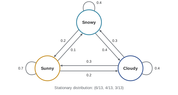
A simple weather model for a prairie city: each day is sunny (S), cloudy (C) or snowy (W, for winter weather). If today is sunny, tomorrow is sunny with probability 0.7, cloudy 0.2, snowy 0.1. If cloudy: 0.3, 0.4, 0.3. If snowy: 0.2, 0.4, 0.4. The matrix is

Multi-step transitions: Chapman–Kolmogorov

What is the probability of snow in two days, given sun today? Condition on tomorrow's state with the law of total probability: \(P(X_2 = W \mid X_0 = S) = \sum_k p_{Sk}p_{kW} = 0.7(0.1) + 0.2(0.3) + 0.1(0.4) = 0.17\). In general, the \(n\)-step transition probabilities \(p_{ij}^{(n)} = P(X_n = j \mid X_0 = i)\) satisfy the Chapman–Kolmogorov equations

The \(n\)-step matrix is the \(n\)th power of \(P\). If the initial state has distribution given by a row vector \(\pi_0\), the distribution at time \(n\) is \(\pi_n = \pi_0P^n\). The proof is a direct application of the Markov property: to go from \(i\) to \(j\) in \(m + n\) steps, the chain must be in some state \(k\) at time \(m\), and given that, the remaining \(n\) steps do not depend on how it got to \(k\).

Stationary distributions

A distribution \(\pi\) (a row vector of non-negative entries summing to 1) is stationary if \(\pi P = \pi\): if the chain starts in \(\pi\), it stays in \(\pi\) forever. For the weather chain, the equations are \(\pi_S = 0.7\pi_S + 0.3\pi_C + 0.2\pi_W\), \(\pi_C = 0.2\pi_S + 0.4\pi_C + 0.4\pi_W\), and \(\pi_S + \pi_C + \pi_W = 1\) (the third balance equation is redundant). The first gives \(0.3\pi_S = 0.3\pi_C + 0.2\pi_W\), and the second gives \(0.6\pi_C = 0.2\pi_S + 0.4\pi_W\). Solving, \(\pi_W = (3/2)(\pi_S - \pi_C)\) from the first; substituting into the second gives \(0.6\pi_C = 0.2\pi_S + 0.6\pi_S - 0.6\pi_C\), so \(\pi_C = (2/3)\pi_S\) and \(\pi_W = (1/2)\pi_S\). Normalizing, \(\pi_S(1 + 2/3 + 1/2) = 1\), so

Two theorems explain why this matters. A finite chain is irreducible if every state can be reached from every other, and aperiodic if it does not cycle with a fixed period (a self-loop with positive probability is enough). For an irreducible, aperiodic finite chain, the stationary distribution is unique, and \(\pi_n \to \pi\) from any starting distribution: every row of \(P^n\) converges to \(\pi\). This is the convergence theorem. And the ergodic theorem, a law of large numbers for Markov chains, says that the long-run fraction of time spent in state \(j\) converges to \(\pi_j\) with probability 1, even though the days are not independent. So in the long run, about 46% of days in this model are sunny. A related fact is that the expected return time to state \(j\), starting from \(j\), is \(1/\pi_j\): a sunny day is followed by the next sunny day after an average of \(13/6 \approx 2.17\) days.

The stationary distribution is the idea behind Google's original PageRank algorithm (1998). A random surfer follows a random link from the current page with probability 0.85 and jumps to a uniformly random page otherwise. The jump makes the chain irreducible and aperiodic, and a page's rank is its stationary probability, computed by repeatedly multiplying a vector by the transition matrix, the power method used in the code below.

Absorbing chains and gambler's ruin

Some chains have absorbing states that, once entered, are never left. The questions are then where the chain is absorbed and how long it takes. The classic example is gambler's ruin. A gambler with \(i\) dollars bets one dollar at a time, winning with probability \(p\) and losing with probability \(q = 1 - p\), and stops on reaching 0 (ruin) or \(N\) (the target). Let \(h_i\) be the probability of reaching \(N\) before 0 from \(i\). Conditioning on the first bet gives a first-step equation

Rewrite it as \(p(h_{i+1} - h_i) = q(h_i - h_{i-1})\), so the differences \(d_i = h_i - h_{i-1}\) satisfy \(d_{i+1} = (q/p)d_i\), and \(d_i = (q/p)^{i-1}d_1\). Summing, \(h_i = d_1\sum_{k=0}^{i-1}(q/p)^k\). The condition \(h_N = 1\) fixes \(d_1\). With \(r = q/p\):

In a fair game the chance of doubling your money is exactly the ratio of your stake to the target, which also follows from the fact that a fair game keeps the expected fortune constant: \(E[\text{final}] = Nh_i = i\). In an unfair game the house edge compounds dramatically. At North American roulette, a bet on red wins with probability \(18/38\), so \(r = 20/18\). Starting with 50 dollars and aiming for 100 with one-dollar bets, \(h_{50} = \frac{1 - r^{50}}{1 - r^{100}} = \frac{1}{1 + r^{50}} \approx 0.005\). The chance of doubling up is about 0.5%, compared with 50% in a fair game. Betting the whole 50 dollars at once gives \(18/38 \approx 0.47\). Against an unfavourable game, timid play is the worst strategy. The problem goes back to an exchange between Pascal and Fermat and was solved in general by Christiaan Huygens and later by Jacob Bernoulli and de Moivre.

The expected duration satisfies a similar first-step equation, \(D_i = 1 + pD_{i+1} + qD_{i-1}\) with \(D_0 = D_N = 0\). In the fair case the solution is \(D_i = i(N - i)\): a gambler with 50 dollars aiming for 100 in a fair game expects to play 2,500 bets. You can verify it by substitution: \(1 + \frac12(i+1)(N-i-1) + \frac12(i-1)(N-i+1) = i(N-i)\).

Monte Carlo simulation

Many probabilities and expectations are too hard to compute exactly. Monte Carlo simulation estimates them by generating many independent realizations with a random number generator and averaging. The law of large numbers guarantees that the estimate converges, and the CLT gives its accuracy: with \(n\) independent replications of a quantity with standard deviation \(\sigma\), the standard error is \(\sigma/\sqrt{n}\), so an approximate 95% interval is the estimate \(\pm 1.96s/\sqrt{n}\), with \(s\) the sample standard deviation. The error falls only like \(1/\sqrt{n}\): each extra decimal digit of accuracy costs a hundred times as many replications. The method was named in 1946–1947 by Stanisław Ulam and John von Neumann at Los Alamos, after the Monte Carlo casino, and was run on ENIAC, one of the first electronic computers; Ulam had the idea while estimating the chance of winning a game of solitaire.

Computers produce pseudo-random numbers: deterministic sequences that pass statistical tests of randomness. Python's random module uses the Mersenne Twister (Matsumoto and Nishimura, 1998), with period \(2^{19937} - 1\). Setting a seed, as every code block in this course does, makes a simulation reproducible: the same seed gives the same results, which is essential for checking work. For cryptography a different kind of generator is needed, and Python provides the secrets module for that purpose.

import random, math
from fractions import Fraction
from statistics import mean, stdev

P = [[0.7, 0.2, 0.1], [0.3, 0.4, 0.3], [0.2, 0.4, 0.4]]
names = "SCW"

def matmul(A, B):
    return [[sum(A[i][k] * B[k][j] for k in range(len(B))) for j in range(len(B[0]))] for i in range(len(A))]

P2 = matmul(P, P)
print("P(snow in two days | sun today) =", round(P2[0][2], 4))

# power method: rows of P^n converge to the stationary distribution
Pn = P
for _ in range(50):
    Pn = matmul(Pn, P)
print("row of P^51:", [round(x, 4) for x in Pn[0]], " exact:", [str(Fraction(k, 13)) for k in (6, 4, 3)])

# ergodic theorem: long-run share of sunny days in one simulated path
rng = random.Random(251)
state, counts = 0, [0, 0, 0]
for _ in range(200_000):
    state = rng.choices(range(3), weights=P[state])[0]
    counts[state] += 1
print("long-run shares:", {names[i]: round(c / sum(counts), 4) for i, c in enumerate(counts)})

# gambler's ruin at North American roulette: 50 dollars, target 100
def h(i, N, p):
    r = (1 - p) / p
    return i / N if r == 1 else (1 - r ** i) / (1 - r ** N)
print(f"P(double 50 at roulette, 1-dollar bets) = {h(50, 100, 18 / 38):.5f};  fair game {h(50, 100, 0.5):.2f}")

def play(i, N, p):
    bets = 0
    while 0 < i < N:
        i += 1 if rng.random() < p else -1; bets += 1
    return i == N, bets
games = [play(5, 10, 0.5) for _ in range(20_000)]
print(f"fair game from 5 to 10: P(win) ~ {mean(w for w, b in games):.3f} (0.5), mean bets ~ {mean(b for w, b in games):.2f} (25)")

# Monte Carlo with a confidence interval: second failure among three exponential(mean 5)
xs = [sorted(rng.expovariate(1 / 5) for _ in range(3))[1] for _ in range(100_000)]
m, se = mean(xs), stdev(xs) / math.sqrt(len(xs))
print(f"replacement time ~ {m:.3f} +/- {1.96 * se:.3f} years (exact {25 / 6:.3f})")

P(snow in two days | sun today) = 0.17
row of P^51: [0.4615, 0.3077, 0.2308]  exact: ['6/13', '4/13', '3/13']
long-run shares: {'S': 0.4587, 'C': 0.3098, 'W': 0.2315}
P(double 50 at roulette, 1-dollar bets) = 0.00513;  fair game 0.50
fair game from 5 to 10: P(win) ~ 0.502 (0.5), mean bets ~ 24.97 (25)
replacement time ~ 4.167 +/- 0.019 years (exact 4.167)

The course in one view

The course began with Kolmogorov's three axioms (1933) and built everything from them. Counting gave probabilities for equally likely outcomes. Conditioning gave the multiplication rule, the law of total probability and Bayes' theorem, which revise probabilities in the light of evidence. Random variables turned outcomes into numbers, described by pmfs, densities and cdfs. Expectation and variance summarized them, and linearity of expectation made hard problems easy. The common families (Bernoulli, binomial, geometric, Poisson, uniform, exponential, gamma, normal) model the situations that recur in practice. Joint distributions, covariance and correlation described several variables together. Transformations and MGFs found the distributions of functions and sums. The law of large numbers and the central limit theorem explained why averages are reliable and approximately normal. This lesson combined these tools to study dependence through time and to compute by simulation. The next courses in statistics, stochastic processes, actuarial science and machine learning all build on these foundations.