
MSAZ-311 · Lesson 5 of 12 · 21 min
Star schema design
▶ Video coming soon A video version of this lesson is on the way.
Before the fifth model session, on Tuesday, November 3, Marisol asked Keiko to bring the spreadsheet that fed her old sales report. It was one enormous table: every sales line, with the store name, region, product description, category, supplier, date, month name, fiscal quarter and customer tier repeated on every row. It worked, after a fashion, but every new question meant another column, and a change to a category name meant rewriting years of rows. Marisol drew a box in the middle of the whiteboard and six boxes around it. "This," she said, "is what the warehouse should look like."
Facts and dimensions
A star schema separates measurements from descriptions. A fact table holds the events the business measures, such as sales lines, with numeric columns that can be added up, such as quantity and amount, and keys that point to the dimensions. Dimension tables hold the descriptions used to filter and group those events: stores, products, dates, customers, promotions. Drawn as a diagram, the fact sits in the middle and the dimensions around it, which is where the name comes from.
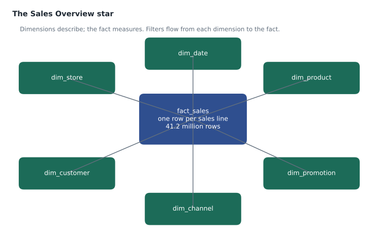
The design is not just tidy; it is what Power BI's engine is built for. Filters on a dimension, such as Region = Prairie, flow along a relationship to the fact table, and the engine compresses dimension columns well because each value is stored once. A star schema also makes measures simpler to write and easier for report authors to understand, because there is one obvious place for each kind of field.
Grain first
The most important decision in a fact table is its grain: what one row represents. Marisol made Keiko write the grain as a sentence before naming any columns: "one row per sales line on a till receipt". Every other choice follows from it. The dimensions are the things that have one value per sales line: one date, one store, one product, one customer (or the non-member customer), one promotion, one channel. The facts are the numbers measured at that grain: quantity, sales amount, discount amount and cost amount.
Mixing grains in one table is the classic error. Keiko's old spreadsheet had a column for the store's monthly target on every sales line, which made summing targets meaningless: a store with 40,000 lines in a month showed a target 40,000 times too big. Targets have a different grain, one row per store per month, so they belong in their own fact table, fact_sales_target, that shares the store and date dimensions with fact_sales.
| Table | Grain | Keys | Measures |
|---|---|---|---|
| fact_sales | One row per sales line | DateKey, StoreKey, ProductKey, CustomerKey, PromotionKey, ChannelKey | Quantity, SalesAmount, DiscountAmount, CostAmount |
| fact_sales_target | One row per store per month | MonthKey, StoreKey | TargetAmount |
| fact_inventory_adjustment | One row per adjustment | DateKey, StoreKey, ProductKey, ReasonKey | QuantityChange, CostChange |
Keys
Dimensions use surrogate keys, the whole-number keys from lesson 3, as their primary keys, and fact tables store those keys. There are three reasons. Surrogate keys make Type 2 history possible, because the same store can have several rows. They insulate the model from source changes, such as StockLine renumbering SKUs. And whole numbers compress and join faster than long text codes. The business key, such as the SKU or store number, stays in the dimension as an ordinary column so people can still search for it.
The date dimension is the exception that people argue about. Many designs use a smart key such as 20261103 for November 3, 2026, because it is readable and sorts correctly, and dates do not change. Keiko used that, and built dim_date with one row per day from January 1, 2019 to December 31, 2030, with columns for the day, month, quarter, the retail fiscal year, which at Harrow & Finch starts on February 1, a flag for statutory holidays and a flag for whether the day is before today.
Dimensions that do more than one job
Some dimensions appear more than once. A sales line has a sale date; a special order also has a promised delivery date. Both point to the same dim_date, which then plays two roles. In the warehouse that is simply two key columns; in the semantic model it means two relationships to one table, only one of which can be active, as lesson 8 explains. A degenerate dimension is a key that has no other attributes, such as the receipt number: it lives in the fact table itself, because a dimension table with only one column would add nothing. A junk dimension gathers small flags, such as "paid by card" and "price overridden", into one small table of their combinations rather than cluttering the fact.
Star or snowflake?
A snowflake schema normalizes dimensions into chains of tables: product to subcategory to category to department. It saves a little space and mirrors the source system, but it adds relationships for the model to follow and for report authors to understand. For Power BI semantic models, Microsoft's guidance favours a star, with each dimension denormalized into one table. Keiko flattened StockLine's four product tables into one dim_product with category and department columns, which is exactly the denormalization step in the DP-600 outline.
# Why a star is smaller than one wide table (rough, illustrative sizes)
fact_rows = 41_200_000
# bytes per row of descriptive text in the old wide table (store, product, category, region, month names...)
wide_text_bytes = 180
key_bytes = 6 * 4                 # six whole-number keys in the fact table
measure_bytes = 4 * 8             # four numeric measures

dims = {"dim_product": (48_000, 160), "dim_store": (27, 120), "dim_date": (4_383, 60),
        "dim_customer": (310_000, 90), "dim_promotion": (900, 70), "dim_channel": (3, 20)}

wide = fact_rows * (wide_text_bytes + measure_bytes)
star = fact_rows * (key_bytes + measure_bytes) + sum(rows * size for rows, size in dims.values())

print(f"Wide table: {wide / 1e9:.1f} GB before compression")
print(f"Star:       {star / 1e9:.1f} GB before compression")
print(f"Star is about {wide / star:.1f} times smaller")Wide table: 8.7 GB before compression Star: 2.3 GB before compression Star is about 3.7 times smaller
What this code does
The example uses the number of sales lines and rough byte sizes for the descriptive text repeated on every row of the old spreadsheet-style table. It compares that with a star, where each fact row holds only six small keys and four numbers and the descriptions are stored once in each dimension. The output shows the wide table at about 8.7 gigabytes against about 2.3 for the star before any compression, so the star is nearly four times smaller, and real compression usually widens the gap further.
The numbers are illustrative, and columnar compression changes them a great deal in practice, because a store name repeated 41 million times compresses very well. The deeper benefit is not size but change: when a category is renamed, the star changes one value in dim_product, and the wide table rewrites every row that mentions it.
Bridge tables
Most relationships in a star are one-to-many: one store has many sales lines. Sometimes the business has a genuine many-to-many relationship. In Finch Rewards, a household can have several members and, since 2025, a member can belong to more than one household, for example a parent who shares points with two adult children. Reporting points earned by household needs a bridge table, bridge_household_member, with one row per member and household pair. Facts link to members, members link to the bridge, and the bridge links to households, so a filter on a household reaches its members' facts. Lesson 8 shows how the semantic model handles the double counting that this can cause when a member is in two households.
Factless facts and snapshots
Two more patterns came up as Keiko listed Grace's other questions. A factless fact table records that something happened with no numbers attached, such as a promotion being active for a product in a store on a day; counting its rows answers "which promotions ran where" and, compared with sales, "which promoted products did not sell". A periodic snapshot records a state at regular intervals, such as stock on hand per product per store each night; snapshots are not additive over time, because adding Monday's stock to Tuesday's means nothing, so their measures must be averaged or taken at the last date of a period.
Worked problem
Choosing a grain for stock on hand
Grace wants to report weekly stock levels and compare them with sales. StockLine records every receipt, sale and adjustment as a movement, about 52,000 a day, and can also produce a nightly snapshot of quantity on hand for about 48,000 SKUs in 23 stores, though only stocked combinations, about 410,000 rows a night. Which fact table should Keiko build, and how big would it be after one year?
Show solution
- A movement fact holds every change; stock on a date is the sum of all movements up to it, which is expensive to compute for every week.
- A nightly snapshot holds the state directly; a weekly report takes the last snapshot in each week.
- Snapshot size: 410,000 rows a night × 365 nights = 149,650,000 rows in a year.
- A weekly snapshot instead would hold 410,000 × 52 = 21,320,000 rows a year and still answer Grace's weekly question.
Answer: A periodic snapshot at weekly grain, about 21.3 million rows a year, with measures that take the last value in a period rather than summing. Keep the movement fact as well if day-level investigations are needed.
Conformed dimensions
Because the hub has several fact tables, the same dimensions have to mean the same thing in each of them. A conformed dimension is one that is shared, with the same keys and attributes, by every fact table that uses it: dim_store and dim_date serve fact_sales, fact_sales_target and fact_inventory_adjustment alike. Conformed dimensions are what make it possible to put sales, targets and shrink side by side in one report and have the store and month filters apply to all three. If the inventory team had built its own store table with different keys, every comparison would need a mapping, and sooner or later two reports would disagree about which stores are in the Prairie region.
Keiko found one place where conformance needed work. StockLine's adjustment records used the old four-digit store codes, while sales used the newer two-digit store numbers. Rather than adding a second store dimension, she added the old code as an attribute of dim_store and looked it up during the adjustment load, so every fact table ended up with the same StoreKey. Marisol called this the quiet work of modelling: nobody sees it in a report, but without it the numbers do not line up.
The date dimension in practice
A date dimension earns its place in almost every model. It turns a plain date into everything people filter by: day of week, week number, month name, the retail fiscal year and quarter, holiday flags and relative flags such as "in the last 13 weeks". Building it once, in the warehouse, means every model and every report uses the same fiscal calendar, which at Harrow & Finch had previously been worked out by hand in three different spreadsheets that did not agree about which week belonged to which quarter. The table is tiny, about 4,400 rows for twelve years, so there is no reason to skimp on columns. In the semantic model it is marked as a date table, which tells Power BI to use it for time intelligence calculations, as lesson 9 shows.
Designing in the warehouse
Keiko created the star in wh_sales with T-SQL: dimensions first, each with its surrogate key, then the fact tables. Fabric warehouses support primary key, foreign key and unique constraints only as NOT ENFORCED declarations; they document the design and help some tools, but the engine does not check them, so the load procedures and the data quality checks from lesson 3 must guarantee that every fact key exists in its dimension. She also wrote the grain sentence for each fact table into the table's description, so that the next person to add a column would see it first.
Common mistakes
MistakePut targets on the sales lines so both are in one table.
InsteadTargets have a different grain; give them their own fact table that shares dimensions.
MistakeUse the source system's codes as the fact table's keys.
InsteadUse surrogate keys in dimensions and facts, and keep business keys as dimension attributes.
MistakeA snowflake is better for Power BI because it is normalized.
InsteadPower BI models work best as stars, with denormalized dimensions.
MistakeSum stock-on-hand snapshots across days.
InsteadSnapshot measures are semi-additive; take the last or average value over time.
Summary and key terms
- A star schema puts measurable events in fact tables and descriptions in dimension tables.
- Decide the grain of each fact table first and write it as a sentence; never mix grains in one table.
- Use surrogate keys; keep business keys as attributes; a date dimension often uses a readable date key.
- Role-playing, degenerate and junk dimensions handle repeated dates, attribute-less keys and small flags.
- Denormalize dimensions into a star; use bridge tables for genuine many-to-many relationships.
- Factless facts record events without numbers; periodic snapshots record states and are semi-additive.
- Fact table
- A table of measurable events at a declared grain, with keys to dimensions.
- Dimension table
- A table of descriptive attributes used to filter and group facts.
- Grain
- What one row of a fact table represents.
- Role-playing dimension
- A dimension used more than once by the same fact, such as order date and delivery date.
- Degenerate dimension
- A dimension key, such as a receipt number, kept in the fact table with no dimension table.
- Bridge table
- A table that resolves a many-to-many relationship between dimensions or between a fact and a dimension.
- Periodic snapshot
- A fact table recording a state, such as stock on hand, at regular intervals.
Practice problems
Work each problem on paper first, then reveal the answer to check.
What should be decided before any columns of a fact table?
Show answer
Its grain: what one row represents.
Why do monthly targets not belong in the sales lines table?
Show answer
They have a different grain, one row per store per month.
What is a degenerate dimension?
Show answer
A key such as a receipt number kept in the fact table without its own dimension table.
Why does Power BI guidance favour stars over snowflakes?
Show answer
Fewer relationships, simpler measures and easier models for report authors.
How should stock-on-hand snapshots be summarized over a month?
Show answer
By the last or average value, not the sum.
Lesson quiz · 5 questions
Score 60% or more to complete this lesson.
Create a free account to save your progress, take quizzes and earn a certificate.