Transforming data with notebooks

Keiko had never written Python for work, and she said so at the start of the fourth model session on Monday, November 2. Marisol said that was fine: the DP-600 exam expects an analytics engineer to read and write simple PySpark, not to be a data engineer, and most of what an analyst does in a notebook is a handful of patterns. Nikolai joined for the first half hour, because the notebook they would write was going to clean the StockLine sales lines that his team had loaded into lh_raw.

Notebooks and Spark in Fabric

A Fabric notebook is an item made of cells. Code cells run in a language chosen per cell, usually PySpark (Python with the Spark library), Spark SQL, Scala or R, and markdown cells hold notes and headings. When the first cell runs, Fabric starts a Spark session on the workspace's Spark pool; the starter pool usually starts in seconds. A notebook attaches to a default lakehouse, whose tables can then be read by name, and it can read other lakehouses and warehouses in OneLake too.

Spark spreads work across many machines, which is why it suits large data, but it also means a notebook is not a spreadsheet. Data lives in DataFrames, which are descriptions of a table and the transformations to apply to it. Most transformations are lazy: nothing runs until an action, such as writing a table, counting rows or displaying a sample, asks for a result. Then Spark plans the whole chain and runs it efficiently.

Reading and looking

The first cells read the raw sales table and looked at it. Marisol insisted on looking before changing anything: the schema, a sample of rows, a count, and the number of nulls in each column.

# PySpark: read the raw sales lines and profile them
from pyspark.sql import functions as F

raw = spark.read.table("lh_raw.stockline_sales_lines")
raw.printSchema()
display(raw.limit(20))
print(raw.count())

nulls = raw.select([F.sum(F.col(c).isNull().cast("int")).alias(c) for c in raw.columns])
display(nulls)

The profile showed three problems. Some rows had a null customer number, which was expected, because not every buyer is a Finch Rewards member. The quantity column was stored as text in one year of extracts. And some transactions appeared more than once, because the till system resent lines after a network drop and the copy had faithfully loaded every resend.

Missing values, types and filters

Missing values need a rule, not a reflex. A null customer number means "not a member", so Keiko replaced it with the value 0, which the customer dimension would map to a "Non-member" row. A null sale amount would have been a real error, so the rule there was to send those rows to a separate quarantine table for investigation rather than filling them. Types were fixed with cast, and rows that could not be converted came out as null, which the quarantine rule then caught. Filters removed test transactions, which StockLine marked with a till number of 999.

clean = (raw
    .filter(F.col("till_no") != 999)                                   # drop test transactions
    .withColumn("quantity", F.col("quantity").cast("int"))            # text to whole number
    .withColumn("customer_no", F.coalesce(F.col("customer_no"), F.lit(0)))
    .withColumn("sku", F.upper(F.trim(F.col("sku")))))

bad  = clean.filter(F.col("amount").isNull() | F.col("quantity").isNull())
good = clean.subtract(bad)

Removing duplicates the right way

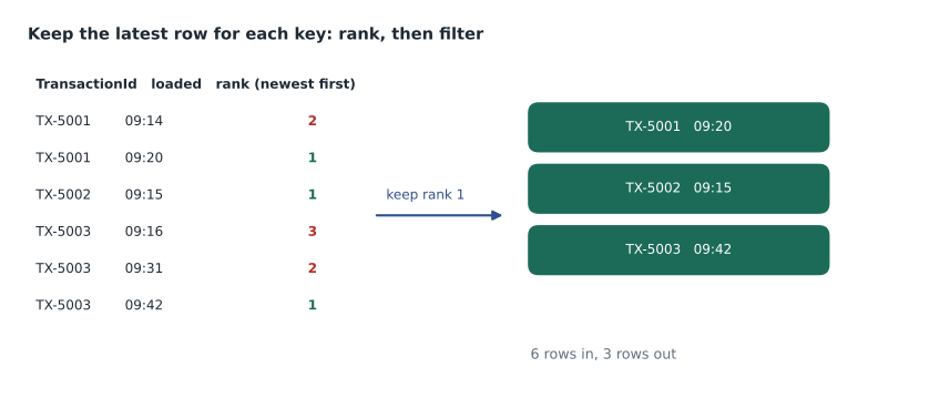
The resent transactions were the interesting problem. dropDuplicates on every column would remove exact copies, but resends were not always exact: the load timestamp differed. dropDuplicates on just the transaction and line number would keep an arbitrary copy. The rule the business wanted was to keep the latest load of each transaction line, because a resend could carry a correction. That needs a window function: rank the rows within each transaction line by load time, newest first, and keep rank 1.

from pyspark.sql.window import Window

w = Window.partitionBy("transaction_id", "line_no").orderBy(F.col("loaded_at").desc())
latest = (good
    .withColumn("rn", F.row_number().over(w))
    .filter(F.col("rn") == 1)
    .drop("rn"))

The same pattern exists in T-SQL, with ROW_NUMBER() OVER (PARTITION BY ... ORDER BY ... DESC), and in Power Query, by grouping and keeping the maximum. Knowing it in all three is useful for the exam, which likes to ask which method removes duplicates while keeping a particular copy. Before running it on 41 million rows, Keiko checked the logic on the example from the figure.

# Keep the newest row for each transaction (the same rule as the window function)
rows = [
    ("TX-5001", "09:14", 182.40), ("TX-5001", "09:20", 172.40),   # resent with a correction
    ("TX-5002", "09:15", 56.10),
    ("TX-5003", "09:16", 18.99), ("TX-5003", "09:31", 18.99), ("TX-5003", "09:42", 18.99),
]

latest = {}
for txn, loaded_at, amount in rows:
    if txn not in latest or loaded_at > latest[txn][0]:
        latest[txn] = (loaded_at, amount)

for txn in sorted(latest):
    print(txn, *latest[txn])
print(len(rows), "rows in,", len(latest), "rows out")
print("Total before:", round(sum(r[2] for r in rows), 2), " after:", round(sum(v[1] for v in latest.values()), 2))

TX-5001 09:20 172.4
TX-5002 09:15 56.1
TX-5003 09:42 18.99
6 rows in, 3 rows out
Total before: 467.87  after: 247.49

The totals line was Marisol's addition. Duplicates do not just make tables bigger; they inflate every sum, and in the real data the resends had overstated two stores' sales by about 0.4 in 100 over three years. Grace's margin question would have been answered with slightly wrong numbers had the duplicates stayed.

Joins and aggregation in PySpark

Joins work as in SQL: df.join(other, on=..., how=...), with how set to inner, left, and so on. Joining the sales lines to the cleaned product table brought in the category, and a left join with a check on the null category found the same 312 unmatched SKUs Keiko had seen in the warehouse. Aggregation uses groupBy and agg, for example daily sales and units by store and product. When one side of a join is small, such as the 23-row store table, Spark can broadcast it to every machine, which avoids moving the large table around; Spark usually does this automatically for small tables.

Spark SQL in the same notebook

Not every cell has to be Python. A cell can switch to Spark SQL with the %%sql magic command at its top, and many analysts find that easier for joins and aggregations. A DataFrame can be registered as a temporary view with createOrReplaceTempView, after which a SQL cell can query it by name, and a SQL query's result can be turned back into a DataFrame with spark.sql. Keiko wrote her daily aggregation in Spark SQL, because it read almost exactly like the T-SQL she knew, and kept the cleaning steps in PySpark, where chaining functions was clearer. Mixing the two is normal; what matters is that each cell is easy for the next reader to follow.

Spark SQL also reads tables in other lakehouses of the workspace by their two-part names, and the notebook's explorer pane lists every attached lakehouse and its tables, so dragging a table into a cell writes the read statement for her. Marisol warned that a notebook attached to the wrong default lakehouse is a common cause of "table not found" errors after deployment, and that the default lakehouse can be set per stage with deployment rules or a variable library, as MSAZ-310 showed.

Reviewing notebook code

Because notebooks are code, Marisol treated them like code. Each notebook in the hub has a markdown cell at the top saying what it reads, what it writes, who owns it and how to rerun it safely. Cells run from top to bottom without hidden state, so that a scheduled run behaves like a manual one; a notebook that only works if cells are run in a special order will eventually fail at 2 a.m. Changes go through Git and a pull request, where another person reads the diff before it reaches Test. And any cell that writes to a table checks its row counts and totals before and after, just as Keiko's warehouse procedures did, so that the notebook fails loudly instead of writing wrong numbers quietly.

Nikolai added one engineering point before he left: use the session sparingly. An idle notebook session keeps a Spark session alive until it times out, and while it is alive it holds capacity. Stopping the session when finished, or letting the scheduled run start and stop its own, keeps the hub's capacity free for the reports that store managers open each morning.

Writing Delta tables

The result was written to lh_curated as a Delta table with saveAsTable. The write mode decides what happens to an existing table: overwrite replaces it, append adds rows, and for incremental updates a Delta MERGE can update matching rows and insert new ones. For the history load Keiko used overwrite; for the nightly run, Nikolai's pipeline would call the notebook with a parameter for the load date, and the notebook would merge that day's rows.

(latest.write
    .mode("overwrite")
    .format("delta")
    .partitionBy("sale_year")
    .saveAsTable("lh_curated.sales_lines"))

Partitioning and file sizes

partitionBy splits a table into folders by a column's values, here one folder per sale year. A query that filters on the partition column reads only the matching folders, which is called partition pruning. Partitioning helps when tables are large and queries usually filter on the column, and it hurts when the column has too many values: partitioning 41 million rows by day would create more than a thousand folders, many with small files, and small files are slow to read. The usual advice is to partition only large tables, on a low-cardinality column that queries filter by, and to keep files reasonably large, in the hundreds of megabytes.

File sizes are their own topic in the outline. Many small appends, such as a load every 15 minutes, leave many small Parquet files. The OPTIMIZE command compacts them, and V-Order, Fabric's Parquet layout optimization, makes reads faster for Power BI and SQL. The lakehouse explorer offers a table maintenance option that runs both, and Fabric can apply optimize-on-write settings to Spark sessions.

Running notebooks on a schedule

A notebook can be scheduled on its own or, more often, run as an activity in a pipeline. A parameters cell, marked as such in the editor, holds default values that the pipeline can override, such as the load date. Each run is recorded in the monitoring hub with its duration and output. Three days after the session, on November 5, a backfill notebook that someone ran by hand during working hours pushed the trial capacity into throttling for about 40 minutes, as MSAZ-310 described; Keiko took from it that heavy notebook runs belong in scheduled windows, not in the middle of the reporting day.