
MSAZ-311 · Lesson 3 of 12 · 21 min
Transforming data with SQL
▶ Video coming soon A video version of this lesson is on the way.
On Thursday, October 29, the third model session moved to the wh_sales warehouse, where the hub's star schema would live. Keiko had written T-SQL for years against StockLine, but always to read data. Marisol wanted her to write the code that builds tables: cleaning products and stores, keeping history when a store changes region, and loading the fact table each night. "In a warehouse, SQL is not just for questions," she said. "It is how the tables get made."
Where T-SQL runs in Fabric
Two Fabric items accept T-SQL. A warehouse is fully read and write: tables can be created, loaded, updated and deleted with T-SQL, and several tables can change in one transaction. A lakehouse's SQL analytics endpoint is read-only for table data, but it supports views, inline table-valued functions and stored procedures that read data, and it can grant SQL permissions on them. Both store tables as Delta in OneLake, and a warehouse can read lakehouse tables in the same workspace with three-part names, such as lh_curated.dbo.products, so a warehouse procedure can pull cleaned data from the lakehouse and write the star schema.
| Task | Warehouse | Lakehouse SQL analytics endpoint |
|---|---|---|
| SELECT, joins, aggregation | Yes | Yes |
| Views and inline functions | Yes | Yes |
| CREATE TABLE, INSERT, UPDATE, DELETE | Yes | No; tables are written by Spark, pipelines or dataflows |
| CREATE TABLE AS SELECT (CTAS) | Yes | No |
| Multi-table transactions | Yes | No |
| Stored procedures | Yes, including ones that write | Yes, for reading only |
Cleaning with views first
Marisol's habit was to write cleaning logic as a view before turning it into a table. A view is just a saved query, so it can be changed in seconds and checked against the source, and only when the logic is right does it become a table that a procedure loads. Keiko's first view cleaned StockLine's product table: trimming SKUs, replacing blank category names with "Unassigned", converting the pack size from text to a whole number, and keeping only active products.
CREATE VIEW stg.v_products AS
SELECT
    UPPER(LTRIM(RTRIM(p.sku)))                     AS Sku,
    p.description                                  AS ProductName,
    COALESCE(NULLIF(LTRIM(RTRIM(p.category)), ''), 'Unassigned') AS Category,
    TRY_CAST(p.pack_size AS int)                   AS PackSize,
    p.modified_at                                  AS ModifiedAt
FROM lh_curated.dbo.stockline_products AS p
WHERE p.is_active = 1;
Three functions do most of the cleaning work. COALESCE returns the first non-null value in its list, so it replaces nulls with a default. NULLIF turns a value into a null when it equals something, here an empty string, so that COALESCE can catch it too. TRY_CAST converts a value and returns null instead of failing when it cannot, which is safer than CAST on messy data; Keiko added a check afterwards that counted the nulls TRY_CAST produced, and found 14 products whose pack size had been typed as "12 pk".
Building tables with CTAS
CREATE TABLE AS SELECT, or CTAS, creates a new table from a query's result in one statement. It is the quickest way to materialize a view, and it is efficient in the warehouse because it writes the new table's files in parallel. A common pattern for full rebuilds is to create the new version of a table with CTAS under a temporary name, check it, and then swap it in with a rename, so that readers never see a half-built table.
CREATE TABLE dbo.dim_product_new AS
SELECT ROW_NUMBER() OVER (ORDER BY Sku) AS ProductKey, Sku, ProductName, Category, PackSize
FROM stg.v_products;

-- after checking row counts and nulls:
EXEC sp_rename 'dbo.dim_product', 'dim_product_old';
EXEC sp_rename 'dbo.dim_product_new', 'dim_product';
The ProductKey column is a surrogate key: a meaningless whole number that identifies each row of the dimension, separate from the business key, the SKU. Lesson 5 explains why star schemas use surrogate keys. Rebuilding with ROW_NUMBER, though, gives products new keys whenever the order of SKUs changes, which would break the fact table's links; for dimensions that grow, the key must be assigned once and kept. Keiko changed the procedure to keep existing keys and number only new SKUs from the current maximum plus one.
Slowly changing dimensions
Dimension attributes change. A store moves from the West region to a new Prairie region; a product is moved to a different category; a customer changes Rewards tier. A slowly changing dimension, or SCD, is the rule for what the dimension does when that happens, and the DP-600 outline names the two that matter most.
Type 1 overwrites the old value. It is simple, and right when the old value was a mistake or when nobody needs history: a corrected product name should simply replace the misspelled one. Type 2 keeps history: the current row is closed by setting an end date and a current flag to false, and a new row with a new surrogate key is added with the new value. Facts recorded before the change keep pointing at the old row, so a report of last year's sales by region still shows the old region, which is what the business usually expects.
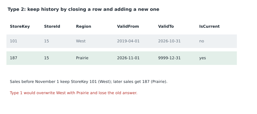
The hub needed Type 2 for exactly that case. On November 1, 2026, Store 15 and three others were moving from the West region to a new Prairie region, and Grace wanted last quarter's margin reported under the regions as they were then. Keiko wrote the change as two statements in one transaction, so that the dimension could never be left with the old row closed and no new row added.
BEGIN TRANSACTION;

UPDATE d SET ValidTo = '2026-10-31', IsCurrent = 0
FROM dbo.dim_store AS d
JOIN stg.v_stores  AS s ON s.StoreId = d.StoreId
WHERE d.IsCurrent = 1 AND s.Region <> d.Region;

INSERT INTO dbo.dim_store (StoreKey, StoreId, StoreName, Region, ValidFrom, ValidTo, IsCurrent)
SELECT (SELECT MAX(StoreKey) FROM dbo.dim_store) + ROW_NUMBER() OVER (ORDER BY s.StoreId),
       s.StoreId, s.StoreName, s.Region, '2026-11-01', '9999-12-31', 1
FROM stg.v_stores AS s
WHERE NOT EXISTS (SELECT 1 FROM dbo.dim_store AS d
                  WHERE d.StoreId = s.StoreId AND d.IsCurrent = 1);

COMMIT TRANSACTION;
The insert's NOT EXISTS test is what makes the two statements work together: after the update, a store whose region changed no longer has a current row, so it qualifies for a new one, and a store that did not change still has its current row and is skipped. The same logic is easy to check on a few rows in Python before running it against the warehouse.
# Apply a Type 2 change to a tiny store dimension
dim = [
    {"key": 101, "store": 15, "region": "West", "from": "2019-04-01", "to": "9999-12-31", "current": True},
    {"key": 102, "store": 16, "region": "West", "from": "2019-04-01", "to": "9999-12-31", "current": True},
]
source = {15: "Prairie", 16: "West"}        # store 15 moves, store 16 does not
change_date, day_before = "2026-11-01", "2026-10-31"

for row in dim:                              # step 1: close rows whose region changed
    if row["current"] and source[row["store"]] != row["region"]:
        row["to"], row["current"] = day_before, False

next_key = max(r["key"] for r in dim) + 1
for store, region in source.items():         # step 2: add a row where none is current
    if not any(r["store"] == store and r["current"] for r in dim):
        dim.append({"key": next_key, "store": store, "region": region,
                    "from": change_date, "to": "9999-12-31", "current": True})
        next_key += 1

for r in dim:
print(r["key"], r["store"], r["region"], r["from"], r["to"], r["current"])101 15 West 2019-04-01 2026-10-31 False 102 16 West 2019-04-01 9999-12-31 True 103 15 Prairie 2026-11-01 9999-12-31 True
What this code does
The example starts with a dimension holding two current store rows and a source that says Store 15 has moved to Prairie while Store 16 has not. First it closes any current row whose region no longer matches the source, giving it an end date of October 31. Then it adds a new current row, with the next key, for any store left without one. The output shows Store 15 with a closed West row and a new Prairie row keyed 103, and Store 16 unchanged.
Joining, aggregating and de-aggregating
Other transformations in the outline come up constantly. Joins combine tables, and the choice between an inner join, which keeps only matching rows, and a left join, which keeps every row from the first table, decides whether unmatched sales disappear or appear with a null product. Keiko always ran both and compared the counts: in the first fact load, 312 sales lines had SKUs missing from the product dimension, and an inner join would have dropped them silently. The fix was an "unknown product" row in dim_product with key -1, so those sales stayed in the totals and showed up in a data quality report.
Aggregation reduces detail with GROUP BY, for example from sales lines to daily sales by store and product, which can make a table hundreds of times smaller for reports that never need line detail. De-aggregation goes the other way, spreading a monthly target across days or stores by a weighting, and it needs care so that the parts add back exactly to the whole. Denormalizing copies attributes into one wider table, such as putting the category name into the product dimension rather than keeping a separate category table, which is exactly what a star schema's dimensions do.
Worked problem
Spreading a monthly target
Grace's team sets Store 12 a paint sales target of 90,000 dollars for November 2026. Keiko must spread it across the four weeks of the month in proportion to last November's weekly paint sales of 18,000, 21,000, 24,000 and 27,000 dollars, and the four weekly targets must add up to exactly 90,000.
Show solution
- Last November's total is 18,000 + 21,000 + 24,000 + 27,000 = 90,000 dollars.
- Each week's share is its sales divided by the total: 0.20, about 0.2333, about 0.2667 and 0.30.
- Multiply each share by the target: 18,000, 21,000, 24,000 and 27,000 dollars.
- Check the sum: 18,000 + 21,000 + 24,000 + 27,000 = 90,000, so nothing is lost to rounding.
Answer: Weekly targets of 18,000, 21,000, 24,000 and 27,000 dollars. When shares do not divide evenly, round all but the last week and give the last week the remainder so the total stays exact.
Stored procedures and scheduling
Once each step worked, Keiko wrapped them in stored procedures: one for each dimension and one for the nightly fact load. A pipeline then runs the procedures in order after Ines's copy activities finish, with a failure path that sends a message to the team channel. Keeping the logic in procedures, rather than in dozens of pipeline activities, means it can be read in one place, versioned through the warehouse's Git integration, and tested in the Test workspace before deployment.
Performance in the warehouse
The warehouse engine handles most queries well without tuning, but a few habits help. Select only the columns needed, because the files are columnar and unread columns cost nothing. Filter early, especially on dates. Load in large batches with CTAS, INSERT ... SELECT or COPY INTO rather than many single-row inserts, which create many small files and log entries. And check the query insights views, which keep a history of recent queries with their durations, to find the slow ones before users do.
Testing belongs in the same habit. Before each procedure ran in Test, Keiko wrote three checks that she now runs after every load: the fact table's row count for the day matches the copied source rows, no fact row has a null key, and the total sales amount for the day matches StockLine's own end-of-day total to the cent. If any check fails, the procedure raises an error and the pipeline stops before the semantic model is refreshed, so store managers see yesterday's correct numbers rather than today's wrong ones.
Common mistakes
MistakeTRY_CAST and CAST behave the same.
InsteadCAST fails the whole statement on a bad value; TRY_CAST returns null, which must then be counted and handled.
MistakeROW_NUMBER over the whole table is a safe way to assign surrogate keys on every load.
InsteadKeys must stay stable; assign new keys only to new rows, starting after the current maximum.
MistakeType 2 is always better than Type 1.
InsteadType 1 suits corrections and attributes nobody tracks over time; Type 2 suits attributes whose history matters.
MistakeAn inner join is fine for loading facts.
InsteadAn inner join silently drops facts with unknown keys; use an unknown member row so they stay visible.
Summary and key terms
- Warehouses accept full T-SQL writes and transactions; lakehouse SQL endpoints are read-only for data but support views and functions.
- Write cleaning logic as views first, using COALESCE, NULLIF and TRY_CAST, then materialize it.
- CTAS creates a table from a query efficiently; swap rebuilt tables in with a rename.
- Type 1 overwrites; Type 2 closes the current row and adds a new one with a new surrogate key, in one transaction.
- Compare inner and left join counts, and use an unknown member for unmatched keys.
- Wrap logic in stored procedures run by a pipeline, and load in batches for performance.
- CTAS
- CREATE TABLE AS SELECT: creating a table from the result of a query.
- Surrogate key
- A meaningless whole-number key that identifies a dimension row, separate from the business key.
- Business key
- The identifier used by the source system, such as a SKU or store number.
- Slowly changing dimension
- A rule for how a dimension handles changes to its attributes.
- Type 1 SCD
- Overwriting an attribute, keeping no history.
- Type 2 SCD
- Keeping history by closing the current row and adding a new row with a new surrogate key.
- Unknown member
- A dimension row, often with key -1, used for facts whose key has no match.
Practice problems
Work each problem on paper first, then reveal the answer to check.
Which Fabric item accepts T-SQL INSERT and UPDATE on its tables?
Show answer
The warehouse.
What does TRY_CAST return when a value cannot be converted?
Show answer
Null.
In a Type 2 change, what happens to the old row?
Show answer
It is closed with an end date and its current flag set to false.
Why compare inner and left join row counts when loading facts?
Show answer
To find facts whose keys have no match before an inner join drops them.
Why put the Type 2 update and insert in one transaction?
Show answer
So the dimension is never left with a store that has no current row.
Lesson quiz · 5 questions
Score 60% or more to complete this lesson.
Create a free account to save your progress, take quizzes and earn a certificate.