Precise point positioning

The canal's western end lay 60 km from the nearest permanent station and well outside comfortable RTK range. Ruth Albrecht wanted two new control points there, CR7 and CR8, with centimetre accuracy in NAD83(CSRS) and no base receiver tied up for a week. Theo Martel set up a geodetic receiver on each for eight hours and uploaded the files to NRCan's CSRS-PPP service the next morning. The reports came back in minutes, each with coordinates, uncertainties of a few millimetres, and a plot showing the solution converging over the first hour. This lesson explains precise point positioning (PPP): how a single receiver, with nothing but precise satellite products, can position itself to centimetres or better anywhere on Earth.

The idea

Relative positioning removes satellite orbit and clock errors by differencing with a base. PPP removes them instead by replacing the broadcast orbits and clocks with precise ones estimated from a global network, as described in Lesson 3. With orbits good to a few centimetres and clocks good to a few hundredths of a nanosecond, the remaining unknowns of an undifferenced dual-frequency observation are the receiver's coordinates, its clock, the tropospheric delay and the carrier-phase ambiguities. A PPP processor forms ionosphere-free combinations of code and phase,

after applying the precise satellite clock, a hydrostatic delay model and many corrections, and estimates the coordinates, the receiver clock at every epoch, the zenith wet delay \(Z_w\) as a slowly varying parameter, and one ambiguity per satellite pass, usually in a Kalman filter or a sequential least-squares adjustment. The code observations pin the clock and give a rough position; the phase observations, once their ambiguities are well determined, give the precision.

What has to be modelled

Because nothing is differenced away, every effect that relative positioning cancels over a short baseline must be modelled explicitly, at the millimetre level. The list is long: satellite antenna phase centre offsets and variations, which are large because the satellite's centre of mass, to which precise orbits refer, is up to a few metres from its antenna; receiver antenna calibrations; phase wind-up as the satellites rotate; the relativistic clock and path effects; solid Earth tides, ocean tide loading and the pole tide; and the satellite attitude, which determines the direction of the antenna offsets and changes rapidly when satellites pass through the Earth's shadow. The models are set out in the conventions of the International Earth Rotation and Reference Systems Service and the standards of the IGS, and the precise products and the PPP software must use consistent conventions: the satellite clocks estimated by an analysis centre absorb its modelling choices, so mixing products and models from different sources can bias results.

Convergence

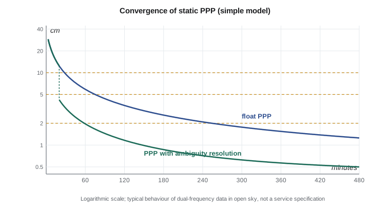
The weakness of float PPP is the time it needs. Each ionosphere-free ambiguity is separated from the coordinates and the troposphere only by the slow change of satellite geometry, so the solution starts at the decimetre-to-metre level of the code and improves gradually. Typical dual-frequency static float PPP reaches about 10 cm horizontally in 20 to 30 minutes and a few centimetres after one to two hours, and millimetre-level precision needs many hours. Heights converge more slowly than horizontal positions. Kinematic PPP converges similarly but with more noise, and any loss of lock on many satellites restarts the convergence.

Ambiguity resolution in PPP

In relative positioning the double-differenced ambiguities are integers because receiver and satellite phase biases cancel. In undifferenced PPP the biases do not cancel: the estimated ambiguity is the integer plus a fractional satellite bias and a fractional receiver bias. Since about 2008 several groups have shown how to estimate the satellite phase biases from a global network and distribute them, either as separate bias products or built into integer-recovery clocks, so that a user can remove them. The receiver bias is common to all satellites and cancels when differences between satellites are formed in the user's filter. The ambiguities can then be fixed, typically with the wide-lane, narrow-lane cascade of Lesson 7. This is PPP with ambiguity resolution (PPP-AR). It improves the east component especially, because float ambiguities correlate most strongly with east–west position, and it shortens the time needed to reach a given accuracy.

PPP-RTK goes further by adding precise ionospheric and tropospheric corrections from a regional network, so that the user can fix ambiguities almost instantly, like RTK, while the correction stream remains compact and valid over a wide area. Several commercial services and the Japanese QZSS centimetre-level service work in this way.

The program below uses a simple convergence model, fitted to the general behaviour of dual-frequency static PPP rather than to any particular service, to compare float PPP with PPP-AR, and to find the time each takes to reach 10, 5 and 2 cm. It then addresses the second practical issue of PPP: bringing the result to the epoch of the national frame.

# PPP convergence (simple model) and bringing a PPP result to the reference epoch
import math

def sigma_h(t_min, ar=False):
    """Horizontal 1-sigma (m) of a static float PPP solution after t minutes: a convergence model
    fitted to typical dual-frequency results; ambiguity resolution removes most of the slow tail."""
    floor, s0, tau = 0.004, 0.40, 6.0
    s = math.sqrt(floor ** 2 + s0 ** 2 * (tau / (t_min + tau)) ** 1.6)
    if ar and t_min >= 20:
        s = math.sqrt(floor ** 2 + (0.35 * (s - floor)) ** 2)
    return s

print("minutes  float PPP (cm)  with ambiguity resolution (cm)")
for t in (5, 10, 20, 30, 60, 120, 240, 480, 1440):
    print(str(t).rjust(7), format(100 * sigma_h(t), "12.1f"), format(100 * sigma_h(t, True), "18.1f"))
for target in (0.10, 0.05, 0.02):
    t = next(t for t in range(1, 3000) if sigma_h(t) <= target)
    ta = next(t for t in range(1, 3000) if sigma_h(t, True) <= target)
    print("time to", int(100 * target), "cm:", t, "min float,", ta, "min with AR")

# After the PPP result is transformed from the global frame to the national frame at the observation
# epoch, it must still be moved to the national frame's reference epoch with the station velocity
obs_epoch, ref_epoch = 2026.84, 2010.0
v_enu = (-0.5, -0.4, 0.9)          # station velocity in the national frame (mm/yr), from a velocity model
dt = ref_epoch - obs_epoch
shift = [v * dt for v in v_enu]
print("epoch change", round(dt, 2), "yr: shift east", round(shift[0], 1), "mm, north", round(shift[1], 1), "mm, up", round(shift[2], 1), "mm")

minutes  float PPP (cm)  with ambiguity resolution (cm)
      5         24.6               24.6
     10         18.3               18.3
     20         12.4                4.2
     30          9.5                3.2
     60          5.9                2.0
    120          3.5                1.2
    240          2.1                0.7
    480          1.3                0.5
   1440          0.6                0.4
time to 10 cm: 28 min float, 20 min with AR
time to 5 cm: 76 min float, 20 min with AR
time to 2 cm: 255 min float, 59 min with AR
epoch change -16.84 yr: shift east 8.4 mm, north 6.7 mm, up -15.2 mm

In the model, float PPP needs about half an hour to reach 10 cm and more than an hour to reach 5 cm; ambiguity resolution, once possible after about 20 minutes, brings the solution to 5 cm at once and to 2 cm within an hour. After a full day both approaches reach a few millimetres. The times are typical rather than guaranteed: open sky, a good antenna and quiet ionospheric conditions shorten them; obstructions and storms lengthen them. The second part of the output is the subject of the next section.

Frames and epochs

Precise orbits are expressed in the frame of the IGS, IGS20, which is aligned with ITRF2020, and they place the satellites where they are today. A PPP solution is therefore in ITRF2020 at the epoch of observation. The North American plate moves about 2 to 3 cm per year relative to the ITRF, so ITRF coordinates of a fixed pillar in Alberta or Montana change every year. National frames such as NAD83 are fixed to the plate, so that points on stable ground keep nearly constant coordinates. To deliver a result in the national frame, the PPP coordinates are transformed from ITRF2020 to the national frame at the observation epoch, using published transformation parameters and their rates, and then moved from the observation epoch to the national frame's reference epoch using the station velocity in that frame.

In Canada the reference epoch for NAD83(CSRS) is 2010.0, and the velocities come from NRCan's velocity grid, which captures the slow motions of the North American plate interior, mainly glacial isostatic adjustment. In the Lethbridge area these are a millimetre or so per year horizontally and vertically. Over 16.84 years the program's example velocities move the pillar by 8 mm east, 7 mm north and 15 mm vertically, enough to matter for control. Leaving the epoch unspecified is one of the most common causes of centimetre-level disagreement between surveys.

Online PPP services

NRCan's CSRS-PPP service is free and accepts RINEX files from anywhere in the world, static or kinematic, single or dual frequency. It returns coordinates in ITRF2020 and, for Canadian users, in NAD83(CSRS) at the reference epoch the user chooses, with uncertainties, residual plots and a full report. Version 5, released in May 2025, added Galileo to the PPP-AR processing, previously GPS and GLONASS, for data processed with rapid or final products, and reported accuracy gains of up to 40 to 60 % for sessions of an hour or less. It chooses the best available product automatically: ultra-rapid products hourly, rapid products about 17 to 18 hours after the end of the day, and final products about two weeks after the end of the week. For control work it is good practice to reprocess with final products once they are available.

Real-time PPP

Real-time PPP uses orbit and clock corrections streamed over the internet or by satellite, such as the IGS real-time service, Galileo's High Accuracy Service and commercial services, in the RTCM state space representation (SSR) format, which describes errors per satellite rather than as base observations. Accuracy after convergence is a few centimetres to a decimetre depending on the service, and convergence takes minutes to tens of minutes. Real-time PPP serves precision agriculture, offshore work, machine guidance far from networks, and the positioning of remote sites. For a surveyor its main weakness is the convergence time after each outage, which makes it awkward for stop-and-go work in obstructed areas.

Using PPP well

PPP is now often the simplest way to establish accurate control far from other control, to check a network, or to coordinate an RTK base. A few practices make it reliable. Observe long enough: several hours for millimetre-level static control, and never less than about an hour for centimetre work. Use a geodetic antenna whose calibration is known to the service, enter its standard name and height exactly, and submit dual-frequency data at 30 s or 1 s intervals. Process with final products for control. Check that the solution has converged, using the convergence plot and the reported uncertainty, and compare two independent sessions on different days. And state the frame and epoch of every coordinate delivered.