Carrier phase and ambiguity resolution

The canal's control network needed relative accuracies of about 5 mm horizontally and 10 mm vertically between points a few kilometres apart, because the canal drops only 0.25 m per kilometre and the hydraulic design was sensitive to the grades. No code measurement can deliver that. Ruth Albrecht set up static sessions of two hours on each pair of points and explained to Leah Tran that the whole method depends on one property of the carrier phase: it measures range in units of 19 cm, and if the receiver can work out exactly how many whole wavelengths separate it from each satellite, its millimetre precision becomes millimetre accuracy. Finding those whole numbers is ambiguity resolution, and this lesson is about how it is done and how to tell when it has gone wrong.

The carrier phase observation

In cycles, the carrier phase measured by receiver \(r\) from satellite \(s\) on one frequency is

where \(\lambda\) and \(f\) are the wavelength and frequency, \(N\) is the integer ambiguity and \(\delta\) are phase hardware delays in cycles. A receiver can measure \(\phi\) to about a hundredth of a cycle, two millimetres, but every term except the noise has to be known or eliminated before that precision can be used. Relative positioning eliminates most of them by differencing observations from two receivers that track the same satellites at the same time.

Single, double and triple differences

The single difference between receivers \(A\) and \(B\) for satellite \(j\), \(\phi_{AB}^j = \phi_B^j - \phi_A^j\), cancels the satellite clock and the satellite hardware delay, and largely cancels orbit and atmospheric errors when the receivers are close. It still contains both receiver clocks. The double difference subtracts two single differences to satellites \(j\) and \(k\):

Both receiver clocks and all receiver hardware delays cancel, because they are the same for satellites \(j\) and \(k\) at each receiver. What remains is the double-differenced range, small residual atmospheric terms that grow with the baseline length, noise, and the double-differenced ambiguity, which is an integer because it is a sum and difference of four integers. Double differences are the standard observable of baseline processing: a session with \(n\) satellites provides \(n - 1\) independent double differences per epoch, all usually referred to one reference satellite, often the highest.

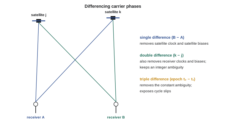
The triple difference subtracts double differences at consecutive epochs. Because the ambiguity is constant while tracking continues, it cancels, leaving only the change in geometry. Triple differences give a rough, ambiguity-free solution useful as a starting point and are sensitive to cycle slips, which appear as an isolated spike, so they are used to find and repair slips before the main solution.

The program below builds phase observations for two receivers and two satellites with large clock errors and arbitrary integer ambiguities, and confirms that after double differencing the phase minus the geometric term is exactly the integer combination of ambiguities.

# Double differences cancel clocks; then fix the float ambiguities to integers
import math, random, itertools
random.seed(11)
lam = 0.1903                                   # L1 wavelength, m

# 1. Clock terms vanish in a double difference
rho = {("B", 1): 20512345.678, ("B", 2): 21877001.234, ("R", 1): 20512301.112, ("R", 2): 21877050.991}
dt_rx = {"B": 3.1e-4, "R": -7.4e-5}; dt_sat = {1: 2.2e-5, 2: -1.6e-5}; c = 299792458.0
N = {("B", 1): 107791234, ("B", 2): 114962875, ("R", 1): 107791001, ("R", 2): 114963140}
phase = {k: rho[k] / lam + c * (dt_rx[k[0]] - dt_sat[k[1]]) / lam + N[k] for k in rho}   # cycles
dd_obs = (phase["R", 2] - phase["B", 2]) - (phase["R", 1] - phase["B", 1])
dd_geom = ((rho["R", 2] - rho["B", 2]) - (rho["R", 1] - rho["B", 1])) / lam
dd_N = (N["R", 2] - N["B", 2]) - (N["R", 1] - N["B", 1])
print("double-difference phase minus geometry:", round(dd_obs - dd_geom, 6), "cycles; integer ambiguity", dd_N)

# 2. Float solution of three double-difference ambiguities and its covariance (cycles^2)
true = [4, -7, 12]
Q = [[0.090, 0.071, 0.052], [0.071, 0.081, 0.047], [0.052, 0.047, 0.065]]
L = [[0.0] * 3 for _ in range(3)]               # Cholesky factor to draw correlated errors
for i in range(3):
    for j in range(i + 1):
        s = sum(L[i][k] * L[j][k] for k in range(j))
        L[i][j] = math.sqrt(Q[i][i] - s) if i == j else (Q[i][j] - s) / L[j][j]
def inv3(A):
    a, b, c_, d, e, f, g, h, i = A[0] + A[1] + A[2]
    det = a * (e * i - f * h) - b * (d * i - f * g) + c_ * (d * h - e * g)
    return [[(e * i - f * h) / det, (c_ * h - b * i) / det, (b * f - c_ * e) / det],
            [(f * g - d * i) / det, (a * i - c_ * g) / det, (c_ * d - a * f) / det],
            [(d * h - e * g) / det, (b * g - a * h) / det, (a * e - b * d) / det]]
W = inv3(Q)
def norm(x, z): d = [a - b for a, b in zip(x, z)]; return sum(d[i] * W[i][j] * d[j] for i in range(3) for j in range(3))

def bootstrap(x):
    x = list(x); out = []
    for i in range(3):          # fix one ambiguity, then condition the rest on it
        zi = round(x[i]); out.append(zi); delta = x[i] - zi
        for j in range(i + 1, 3):
            x[j] -= Q[j][i] / Q[i][i] * delta
    return out

def search(x):
    cands = itertools.product(*[range(round(v) - 2, round(v) + 3) for v in x])
    best = sorted(cands, key=lambda z: norm(x, z))[:2]
    return list(best[0]), norm(x, best[1]) / norm(x, best[0])

ok = {"rounding": 0, "bootstrapping": 0, "integer search": 0}; accepted = wrong_accepted = 0
for t in range(2000):
    g = [random.gauss(0, 1) for _ in range(3)]
    x = [true[i] + sum(L[i][k] * g[k] for k in range(3)) for i in range(3)]
    ok["rounding"] += [round(v) for v in x] == true
    ok["bootstrapping"] += bootstrap(x) == true
    z, ratio = search(x); ok["integer search"] += z == true
    if ratio > 3.0:
        accepted += 1; wrong_accepted += z != true
for k, v in ok.items():
    print(k.ljust(15), "success rate", format(100 * v / 2000, "5.1f"), "%")
print("ratio test > 3 accepted", format(100 * accepted / 2000, "4.1f"), "% of epochs;", wrong_accepted, "wrong fixes accepted")

double-difference phase minus geometry: 498.0 cycles; integer ambiguity 498
rounding        success rate  84.5 %
bootstrapping   success rate  88.8 %
integer search  success rate  93.5 %
ratio test > 3 accepted 71.5 % of epochs; 10 wrong fixes accepted

The float solution

With the double-differenced ambiguities treated as real-valued unknowns, a least-squares adjustment of all epochs estimates the baseline components and the ambiguities together. This is the float solution. Its baseline is good to a few centimetres to a decimetre after an hour on a short baseline, but it converges slowly, because the ambiguities are only separated from the coordinates by the slow change of satellite geometry. The float ambiguities are correlated with each other and with the coordinates, often strongly. Their covariance matrix is the key to the next step.

Fixing ambiguities to integers

If the float ambiguities are close enough to their true integer values, fixing them to those integers and re-solving for the coordinates collapses the uncertainty of the baseline to the level of the phase noise, a few millimetres. This is the fixed solution. The difficulty is deciding which integers are correct. Three strategies of increasing sophistication are used.

Rounding each float ambiguity to the nearest integer ignores the correlations and works only when each ambiguity's standard deviation is well below a cycle. Bootstrapping fixes the ambiguities one at a time, most precise first, and after each fix updates the remaining float values using their correlation with the one just fixed; it is better than rounding and simple to compute. Integer least squares finds the vector of integers that minimizes the weighted distance to the float solution,

and is optimal in the sense that it maximizes the probability of fixing correctly. Searching all integer vectors naively is slow when the float ambiguities are strongly correlated, because the search space is a long, thin ellipsoid. The LAMBDA method, published by Peter Teunissen in 1993, transforms the ambiguities by an integer-preserving transformation that decorrelates them, making the search space nearly spherical and the search fast, then transforms the answer back. It is used, in one form or another, in almost every precise GNSS processor.

The simulation in the program draws 2000 float solutions for three correlated double-differenced ambiguities with standard deviations of about 0.25 to 0.30 cycles and correlations near 0.8. Rounding succeeds 84.5 % of the time, bootstrapping 88.8 % and integer search 93.5 %. Even the best method fails on one epoch in fifteen, which is why ambiguity resolution needs validation.

Validation: is the fix right?

A wrong fix is worse than no fix. The coordinates are then biased by a multiple of the wavelength projected onto the baseline, typically several centimetres to decimetres, while the solution reports millimetre precision. Validation tests compare the best integer candidate with the second best. The most widely used is the ratio test: the ratio of the weighted squared distance of the second-best candidate to that of the best must exceed a threshold, commonly 2 or 3. A large ratio means the best candidate is clearly better than any alternative. In the simulation a threshold of 3 accepted 71.5 % of epochs and let through ten wrong fixes out of 2000 trials; a higher threshold would reject more wrong fixes at the cost of accepting fewer correct ones. More rigorous approaches use fixed failure-rate thresholds derived from the success rate computed from the float covariance.

Other practical checks follow. The fixed solution's residuals should be small and random, with a reference variance near one. Repeating the session at a different time, with different satellites, should give the same baseline within a few millimetres. And the baselines of a closed loop of points should sum to nearly zero. Ruth's rule for the canal network was that no baseline was accepted on its fixed solution alone: each point had to be connected by at least two independent baselines, observed in sessions at least a few hours apart.

Making ambiguities easier: wide lanes and multiple frequencies

The difficulty of fixing depends on the ratio of the uncertainty to the wavelength. The wide-lane combination of L1 and L2 has an 86 cm wavelength, and of L1 and L5 75 cm, so its ambiguities are easy to fix, often from a few epochs of the Melbourne–Wübbena combination, which is free of geometry and ionosphere. Once the wide-lane ambiguity \(N_1 - N_2\) is known, the remaining ambiguity can be fixed using the ionosphere-free combination, whose effective wavelength is then about 10.7 cm, the narrow lane. This cascade is standard in long-baseline and PPP processing. With three frequencies, an extra-wide-lane combination of L2 and L5 has a wavelength of almost 6 m and can be fixed almost instantaneously, which shortens convergence further.

Special cases

GLONASS FDMA signals complicate double differences, because each satellite has a different wavelength: the double difference no longer contains a pure integer unless the single-difference ambiguity of the reference satellite is known, and receiver inter-frequency biases differ between brands. Software handles this with calibrated biases or by fixing only part of the GLONASS ambiguities. Galileo, BeiDou and GPS CDMA signals have no such problem, and modern processors often fix them first. Mixing receiver brands at the two ends of a baseline can also cause quarter-cycle or half-cycle offsets between signal components; RTCM messages and processing software correct these when the receiver and antenna are described correctly.

When some ambiguities are poorly determined, for example those of low or recently risen satellites, partial ambiguity resolution fixes only a subset that passes validation and leaves the rest float. This is common in RTK and PPP, where it shortens the time to a usable solution.