Pseudorange positioning

Grant Okonkwo's crew used hand-held receivers to find the old survey markers along the canal route before the precise work began. Their screens showed a position and an accuracy estimate of a few metres, updated every second, with no base station and no post-processing. Leah Tran wanted to know what the receiver was actually doing with its pseudoranges, and why the accuracy figure changed when a truck parked next to the crew. This lesson builds the stand-alone position solution from first principles: the observation equation, its linearization, least-squares estimation, and the dilution of precision that measures how satellite geometry turns range errors into position errors.

Ranging and the clock problem

If a receiver knew the exact range to three satellites at known positions, its position would be at the intersection of three spheres; in practice two intersection points exist, and the one far out in space is easily rejected. But receivers carry inexpensive quartz oscillators, not atomic clocks, and a clock error of one microsecond means a range error of 300 m. Because the same receiver clock error affects every pseudorange measured at the same instant, it can be treated as a fourth unknown, and four pseudoranges give four equations in four unknowns. This was the central idea of GPS: put the expensive clocks in the satellites and let the receiver solve for its own clock.

Dropping the small terms of the observation equation from Lesson 2, and assuming the satellite clock and the atmospheric delays have been corrected from the broadcast message and models, the pseudorange to satellite \(s\) is

with four unknowns, the receiver's ECEF coordinates \(X, Y, Z\) and its clock error \(dt_r\). The equation is nonlinear in the coordinates, so it is solved iteratively by linearizing around an approximate position.

Linearization and least squares

Let \(X_0, Y_0, Z_0\) be an approximate position and \(\rho_0^s\) the range computed from it. A first-order Taylor expansion gives

The coefficients are the components of the unit vector from the satellite toward the receiver. With \(m\) satellites the equations form a linear system \(\mathbf{w} = \mathbf{A}\,\Delta\mathbf{x} + \boldsymbol{\varepsilon}\), where each row of the design matrix \(\mathbf{A}\) is \([-u_x, -u_y, -u_z, 1]\) for the line-of-sight unit vector \(\mathbf{u}\) from receiver to satellite, and \(\mathbf{w}\) is the vector of observed minus computed pseudoranges. When \(m > 4\) the system is overdetermined and the least-squares solution from GEOM-220 applies:

The approximate position is updated by \(\Delta\hat{\mathbf{x}}\) and the process repeated until the corrections are negligible. Remarkably, the iteration converges even from the centre of the Earth, because the unit vectors change slowly with the approximate position: after three or four iterations the corrections fall below a millimetre. Receivers normally start from their last known position and need only one iteration per epoch.

The weight matrix \(\mathbf{W}\) reflects the different quality of the observations. Low-elevation signals pass through more atmosphere and suffer more multipath, so a common model gives each pseudorange a variance proportional to \(1/\sin^2 E\), where \(E\) is the elevation; another weights by measured C/N0. With equal weights \(\mathbf{W} = \mathbf{I}\) and the cofactor matrix of the solution is \(\mathbf{Q} = (\mathbf{A}^{\mathsf T}\mathbf{A})^{-1}\).

Dilution of precision

If every pseudorange has the same independent error with standard deviation \(\sigma\), called the user equivalent range error (UERE), the covariance of the solution is \(\sigma^2 \mathbf{Q}\). The matrix \(\mathbf{Q}\) depends only on geometry, so it measures how geometry dilutes the precision of the ranges. Expressing its position block in local east, north and up coordinates gives the dilution of precision (DOP) factors:

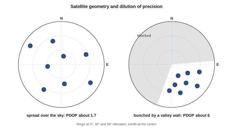
and the standard deviation of, for example, the horizontal position is approximately \(\text{HDOP} \times \sigma\). Good geometry has satellites spread around the sky, some low in every direction and at least one high; poor geometry has satellites bunched together, as in a narrow valley or along a street between tall buildings. VDOP is almost always larger than HDOP, because all satellites are above the horizon: the vertical is constrained only from one side, and the vertical component is correlated with the clock. This is the geometric reason why GNSS heights are less precise than horizontal positions, by a factor of about 1.5 to 2.

A complete solution

The program below places eight satellites at realistic azimuths and elevations around CR1, generates pseudoranges with a receiver clock error of 125 µs (about 37.5 km of range) and 1.5 m of random noise, and solves for position and clock by iterated least squares starting from the centre of the Earth. It then rotates the cofactor matrix into local coordinates and prints the DOP values.

# Least-squares pseudorange positioning with DOP, starting from X = Y = Z = 0
import math, random
random.seed(7)

def ecef(lat, lon, h, a=6378137.0, f=1 / 298.257222101):
    e2 = f * (2 - f); la, lo = math.radians(lat), math.radians(lon)
    N = a / math.sqrt(1 - e2 * math.sin(la) ** 2)
    return [(N + h) * math.cos(la) * math.cos(lo), (N + h) * math.cos(la) * math.sin(lo), (N * (1 - e2) + h) * math.sin(la)]

def enu_rows(lat, lon):
    la, lo = math.radians(lat), math.radians(lon)
    return [[-math.sin(lo), math.cos(lo), 0.0],
            [-math.sin(la) * math.cos(lo), -math.sin(la) * math.sin(lo), math.cos(la)],
            [math.cos(la) * math.cos(lo), math.cos(la) * math.sin(lo), math.sin(la)]]

LAT, LON, H = 49.6967306, -112.8270879, 893.412          # pillar CR1
truth = ecef(LAT, LON, H); R = enu_rows(LAT, LON)
c = 299792458.0; clock = 1.25e-4                         # receiver clock 125 microseconds fast

# Satellites placed at the given azimuth and elevation on a 26 560 km orbit sphere
sky = [(15, 72), (68, 34), (122, 18), (171, 49), (215, 26), (262, 61), (301, 14), (340, 38)]
sats = []
for az, el in sky:
    a, e = math.radians(az), math.radians(el)
    u_enu = [math.cos(e) * math.sin(a), math.cos(e) * math.cos(a), math.sin(e)]
    u = [sum(R[k][i] * u_enu[k] for k in range(3)) for i in range(3)]       # ENU to ECEF
    b = sum(ui * ti for ui, ti in zip(u, truth)); r2 = sum(t * t for t in truth)
    rho = -b + math.sqrt(b * b - r2 + 26560e3 ** 2)
    sats.append([t + rho * ui for t, ui in zip(truth, u)])
P = [math.dist(s, truth) + c * clock + random.gauss(0, 1.5) for s in sats]   # 1.5 m noise

def solve(A, y):   # normal equations by Gaussian elimination
    n = len(A[0]); N = [[sum(A[k][i] * A[k][j] for k in range(len(A))) for j in range(n)] for i in range(n)]
    u = [sum(A[k][i] * y[k] for k in range(len(A))) for i in range(n)]
    M = [N[i] + [u[i]] + [1.0 if i == j else 0.0 for j in range(n)] for i in range(n)]
    for col in range(n):
        p = max(range(col, n), key=lambda r: abs(M[r][col])); M[col], M[p] = M[p], M[col]
        d = M[col][col]; M[col] = [v / d for v in M[col]]
        for r in range(n):
            if r != col:
                f = M[r][col]; M[r] = [a - f * b for a, b in zip(M[r], M[col])]
    return [M[i][n] for i in range(n)], [row[n + 1:] for row in M]

x = [0.0, 0.0, 0.0, 0.0]          # X, Y, Z, c*dt
for it in range(8):
    A, w = [], []
    for s, p in zip(sats, P):
        rho = math.dist(s, x[:3])
        A.append([(x[k] - s[k]) / rho for k in range(3)] + [1.0])
        w.append(p - (rho + x[3]))
    dx, Q = solve(A, w)
    x = [a + b for a, b in zip(x, dx)]
    print("iteration", it + 1, " correction", format(math.sqrt(sum(d * d for d in dx[:3])), "14.3f"), "m")
    if math.sqrt(sum(d * d for d in dx)) < 1e-4:
        break

d = [a - b for a, b in zip(x[:3], truth)]
e, n, u = (sum(R[k][i] * d[i] for i in range(3)) for k in range(3))
print("error east", round(e, 2), "north", round(n, 2), "up", round(u, 2), "m; clock", round(x[3] / c * 1e6, 3), "microseconds")
# Rotate the position block of the cofactor matrix to ENU for HDOP and VDOP
Qx = [r[:3] for r in Q[:3]]
Qenu = [[sum(R[i][a] * Qx[a][b] * R[j][b] for a in range(3) for b in range(3)) for j in range(3)] for i in range(3)]
print("GDOP", round(math.sqrt(sum(Q[i][i] for i in range(4))), 2), " PDOP", round(math.sqrt(sum(Q[i][i] for i in range(3))), 2),
      " HDOP", round(math.sqrt(Qenu[0][0] + Qenu[1][1]), 2), " VDOP", round(math.sqrt(Qenu[2][2]), 2), " TDOP", round(math.sqrt(Q[3][3]), 2))

iteration 1  correction    7558779.819 m
iteration 2  correction    1159866.558 m
iteration 3  correction      32373.785 m
iteration 4  correction         25.259 m
iteration 5  correction          0.000 m
error east -0.07 north -1.4 up 1.49 m; clock 125.003 microseconds
GDOP 1.99  PDOP 1.75  HDOP 0.94  VDOP 1.47  TDOP 0.94

The first correction is more than 7500 km, because the starting point is the centre of the Earth; by the fourth it is 25 m, and the fifth is zero to the printed precision. The clock is recovered to a few nanoseconds of its true 125 µs. The position errors of −0.07 m east, −1.40 m north and +1.49 m up are consistent with the DOP values: with 1.5 m noise and HDOP 0.94, horizontal errors of about 1.4 m are expected, and with VDOP 1.47, vertical errors of about 2.2 m. Running the program with other random seeds shows errors scattered around those sizes.

Multi-GNSS solutions

With several systems, each has its own time scale, so the receiver clock error relative to GPS time differs from that relative to Galileo or BeiDou time by the inter-system time offset plus a receiver hardware bias that differs between signal types. The usual approach estimates one additional parameter per extra system, an inter-system bias, by adding a column to the design matrix with ones for that system's satellites and zeros elsewhere. A four-system solution therefore has seven unknowns and needs at least seven satellites, in practice many more. The improvement in DOP is dramatic where the sky is obstructed: in a coulee bottom with half the sky blocked, GPS alone might show a PDOP of 6 or more, while four systems together often keep it below 2.

What stand-alone positioning delivers

The quality of a stand-alone position is UERE multiplied by DOP. For a single-frequency receiver the UERE is dominated by the residual ionospheric delay after the broadcast model, and is typically 2 to 4 m; for a dual-frequency receiver, which removes the ionosphere with the ionosphere-free combination, it is closer to 1 m, set by broadcast orbit and clock errors and multipath. Typical horizontal accuracy at 95 % confidence is therefore about 3 to 5 m for consumer single-frequency receivers in open sky and 1 to 2 m for dual-frequency receivers. Lesson 5 examines each error source in turn.

The accuracy figure a receiver displays is an estimate, usually computed from DOP and an assumed or measured range error, and sometimes from the residuals of the solution. It describes precision under the receiver's own assumptions. It does not detect a satellite with a bad clock, a reflected signal from the truck beside Grant's crew, or a datum mismatch between the receiver output and the project coordinates. The truck reflected strong signals into the antenna; the multipath added several metres to some pseudoranges and the residuals grew, so the receiver's error estimate rose. Lesson 12 shows how residual tests can detect and exclude a faulty measurement.

Coordinates and the reference frame

The position from a stand-alone receiver is in the frame of the broadcast orbits, WGS 84 for GPS, aligned with the current ITRF at the observation epoch. That is not the same as the national frame used for project coordinates. On this continent the difference between ITRF2020 at the current epoch and NAD83 is about 1.5 to 2 m, mostly a shift of the origin and the motion of the North American plate since 2010. For metre-level work the difference may not matter; for anything better it must be handled, and the frames are revisited in Lessons 9 and 10. A receiver that outputs coordinates labelled simply WGS 84 is giving the frame of the satellites, not of the project.