Satellite orbits

A pseudorange is useless without the position of the satellite that sent it. A 1 m error in a satellite's position along the line of sight goes straight into the range, and through the range into the user's position. Leah Tran had always taken satellite positions for granted; the receiver simply knew them. Ruth Albrecht asked her to compute one by hand from a broadcast navigation message, \"so that you understand what the receiver trusts every second.\" This lesson covers how satellites move, how their orbits are described in the broadcast message and in precise products, and the corrections needed to turn an orbit into a satellite position at the instant a signal left it.

Kepler's laws and the orbital elements

To a first approximation a satellite moves under the gravity of a point mass, and its orbit is a Keplerian ellipse with the centre of the Earth at one focus. Six numbers, the Keplerian elements, fix the ellipse and the satellite's place on it. The semi-major axis \(a\) sets the size and, through Kepler's third law, the period. The eccentricity \(e\) sets the shape; GNSS orbits are nearly circular, with \(e\) usually below 0.02. The inclination \(i\) is the angle between the orbital plane and the equator. The right ascension of the ascending node \(\Omega\) is the direction, measured in the equatorial plane from the vernal equinox, at which the satellite crosses the equator going north. The argument of perigee \(\omega\) is the angle in the orbital plane from the ascending node to the point of closest approach. Finally, the mean anomaly \(M\) at a reference time locates the satellite along the orbit.

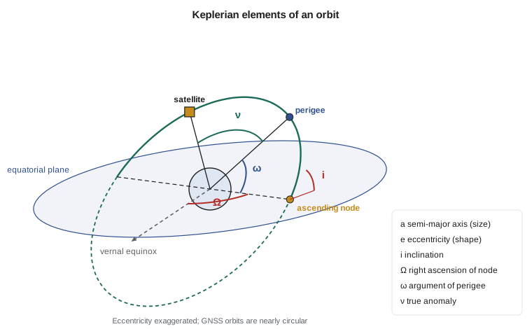
The mean anomaly grows uniformly with time, \(M = M_0 + n(t - t_0)\), where \(n = \sqrt{GM/a^3}\) is the mean motion. It is not an angle you can draw; it is the angle a satellite would have swept out if it moved at constant speed. The eccentric anomaly \(E\) is a geometric angle related to it by Kepler's equation,

which has no closed-form solution for \(E\) but converges in a few iterations of \(E_{k+1} = M + e \sin E_k\) when \(e\) is small. The true anomaly \(\nu\), the actual angle from perigee to the satellite seen from the Earth's centre, and the radius then follow from

Perturbations

Real orbits are not fixed ellipses. The largest perturbation comes from the Earth's equatorial bulge, described by the second zonal harmonic \(J_2\) of the gravity field. It makes the orbital plane precess, so the node drifts westward by about 0.04° per day for GPS orbits, and it makes the perigee rotate within the plane. The Sun and Moon pull on the satellites with accelerations of order \(10^{-6}\ \text{m/s}^2\), and over a few hours they change positions by hundreds of metres. Solar radiation pressure, the push of sunlight on the satellite's large solar panels, is smaller but harder to model because it depends on the satellite's shape, attitude and surface properties, and it changes abruptly when the satellite enters the Earth's shadow. These are the forces that orbit determination must capture to reach centimetre accuracy.

The broadcast ephemeris

Rather than broadcasting a pure Keplerian orbit, GPS, Galileo, BeiDou and QZSS broadcast a quasi-Keplerian ephemeris fitted to the control segment's predicted orbit over a few hours. It has Keplerian elements at a reference time \(t_{oe}\), rates of change of the node and inclination, a correction to the mean motion, and six harmonic correction terms, the amplitudes of sine and cosine terms at twice the argument of latitude for the radius (\(C_{rs}, C_{rc}\)), the argument of latitude (\(C_{us}, C_{uc}\)) and the inclination (\(C_{is}, C_{ic}\)). The receiver evaluates them with the user algorithm published in each system's interface specification. A GPS ephemeris is normally refreshed every two hours and is valid for about four hours around \(t_{oe}\); outside that span its error grows rapidly.

GLONASS takes a different approach. It broadcasts the satellite's position, velocity and lunisolar acceleration in an Earth-fixed frame at a reference time, every 30 minutes, and the receiver integrates the equations of motion numerically, with the \(J_2\) term, to the time required. The result is equivalent, but software must implement both methods.

The broadcast message also carries the satellite clock as a polynomial in time, \(dt^s = a_{f0} + a_{f1}(t - t_{oc}) + a_{f2}(t - t_{oc})^2\), plus a group delay term for single-frequency users. Broadcast orbit and clock errors combined, measured along the line of sight as the signal-in-space range error, are now typically a few decimetres for GPS and Galileo, which is far better than the specifications that were written when the systems were designed.

Computing a satellite position

The algorithm runs as follows. Compute the time from the reference epoch \(t_k = t - t_{oe}\), allowing for week crossovers. Compute the corrected mean motion and the mean anomaly. Solve Kepler's equation for \(E\) and compute the true anomaly. Add the argument of perigee to get the argument of latitude \(\phi\), then apply the second harmonic corrections to obtain the corrected argument of latitude \(u\), radius \(r\) and inclination \(i\). The position in the orbital plane is \((r\cos u, r\sin u)\). Finally, compute the longitude of the ascending node in the Earth-fixed frame, which is the broadcast \(\Omega_0\) plus its rate, minus the Earth's rotation since the start of the GPS week:

and rotate the orbital-plane coordinates into Earth-centred, Earth-fixed (ECEF) coordinates. The program below implements the whole algorithm for one illustrative ephemeris record and then computes the azimuth, elevation and range of the satellite as seen from pillar CR1 over two hours.

# Satellite position from a GPS broadcast ephemeris (the user algorithm of IS-GPS-200)
import math

GM = 3.986005e14            # value fixed by the GPS interface specification
OMEGA_E = 7.2921151467e-5   # Earth rotation rate, rad/s

eph = {  # one broadcast record (illustrative values in the format a receiver decodes)
    "toe": 345600.0, "sqrtA": 5153.6542, "e": 0.0081, "i0": 0.9615, "IDOT": -2.1e-10,
    "OMEGA0": 1.9120, "OMEGADOT": -8.1e-9, "omega": 0.8710, "M0": 0.8150, "dn": 4.6e-9,
    "Cuc": -1.1e-6, "Cus": 7.9e-6, "Crc": 230.5, "Crs": -21.3, "Cic": 1.2e-7, "Cis": -5.6e-8,
}

def sat_xyz(t, p):
    A = p["sqrtA"] ** 2
    n = math.sqrt(GM / A ** 3) + p["dn"]           # corrected mean motion
    tk = t - p["toe"]                              # time from ephemeris reference epoch
    M = p["M0"] + n * tk                           # mean anomaly
    E = M
    for _ in range(10):                            # Kepler's equation by iteration
        E = M + p["e"] * math.sin(E)
    nu = math.atan2(math.sqrt(1 - p["e"] ** 2) * math.sin(E), math.cos(E) - p["e"])
    phi = nu + p["omega"]                          # argument of latitude
    du = p["Cus"] * math.sin(2 * phi) + p["Cuc"] * math.cos(2 * phi)
    dr = p["Crs"] * math.sin(2 * phi) + p["Crc"] * math.cos(2 * phi)
    di = p["Cis"] * math.sin(2 * phi) + p["Cic"] * math.cos(2 * phi)
    u = phi + du
    r = A * (1 - p["e"] * math.cos(E)) + dr
    i = p["i0"] + di + p["IDOT"] * tk
    xo, yo = r * math.cos(u), r * math.sin(u)      # position in the orbital plane
    Om = p["OMEGA0"] + (p["OMEGADOT"] - OMEGA_E) * tk - OMEGA_E * p["toe"]
    return (xo * math.cos(Om) - yo * math.cos(i) * math.sin(Om),
            xo * math.sin(Om) + yo * math.cos(i) * math.cos(Om),
            yo * math.sin(i)), E

def geodetic_to_ecef(lat, lon, h, a=6378137.0, f=1 / 298.257222101):
    e2 = f * (2 - f); la, lo = math.radians(lat), math.radians(lon)
    N = a / math.sqrt(1 - e2 * math.sin(la) ** 2)
    return ((N + h) * math.cos(la) * math.cos(lo), (N + h) * math.cos(la) * math.sin(lo), (N * (1 - e2) + h) * math.sin(la))

def az_el(rx, sat, lat, lon):
    d = [s - r for s, r in zip(sat, rx)]
    la, lo = math.radians(lat), math.radians(lon)
    e = -math.sin(lo) * d[0] + math.cos(lo) * d[1]
    n = -math.sin(la) * math.cos(lo) * d[0] - math.sin(la) * math.sin(lo) * d[1] + math.cos(la) * d[2]
    u = math.cos(la) * math.cos(lo) * d[0] + math.cos(la) * math.sin(lo) * d[1] + math.sin(la) * d[2]
    rng = math.sqrt(e * e + n * n + u * u)
    return math.degrees(math.atan2(e, n)) % 360, math.degrees(math.asin(u / rng)), rng

LAT, LON, H = 49.6967306, -112.8270879, 893.412   # pillar CR1
rx = geodetic_to_ecef(LAT, LON, H)
print("CR1 ECEF (km):", [round(v / 1000, 3) for v in rx])
for dt in (0, 900, 1800, 3600, 7200):
    t = eph["toe"] + dt
    (x, y, z), E = sat_xyz(t, eph)
    az, el, rng = az_el(rx, (x, y, z), LAT, LON)
    print("t - toe =", str(dt).rjust(4), "s  sat (km)", format(x / 1000, "10.3f"), format(y / 1000, "10.3f"), format(z / 1000, "10.3f"),
          " az", format(az, "6.1f"), " el", format(el, "5.1f"), " range", format(rng / 1000, "8.1f"), "km")

# Relativistic clock correction from the eccentricity: dt_r = F e sqrt(A) sin E
F = -4.442807633e-10
(x, y, z), E = sat_xyz(eph["toe"], eph)
print("relativistic clock term at toe:", round(F * eph["e"] * eph["sqrtA"] * math.sin(E) * 1e9, 2), "ns =",
      round(F * eph["e"] * eph["sqrtA"] * math.sin(E) * 299792458, 2), "m")

CR1 ECEF (km): [-1603.878, -3810.431, 4841.72]
t - toe =    0 s  sat (km) -13540.775  -7258.023  21485.609  az  296.5  el  58.7  range  20770.0 km
t - toe =  900 s  sat (km) -12916.445  -9645.242  20951.399  az  290.0  el  65.0  range  20531.5 km
t - toe = 1800 s  sat (km) -12432.223 -11978.309  20051.558  az  277.5  el  70.3  range  20379.1 km
t - toe = 3600 s  sat (km) -11862.791 -16291.127  17227.596  az  230.5  el  72.9  range  20357.4 km
t - toe = 7200 s  sat (km) -11764.989 -22395.430   8299.729  az  188.9  el  49.3  range  21461.8 km
relativistic clock term at toe: -13.57 ns = -4.07 m

At the reference time the satellite is at azimuth 296.5° and elevation 58.7°, about 20,770 km from the pillar. Over the next hour it climbs to 73° and swings round to the south-west, and two hours later it is descending at 49° in the south. The range never drops below about 20,350 km, the altitude plus a little, because the satellite is never directly overhead at this latitude in this pass. The last line shows the relativistic correction caused by the slight eccentricity of the orbit: about −14 ns, or −4 m, at this point of the orbit. Without it the satellite clock would be wrong by up to several metres over each revolution.

Signal travel time and Earth rotation

A signal takes about 67 to 86 ms to reach the ground from a MEO satellite. The satellite position needed is the one at the time of transmission, not the time of reception, so a receiver computes the transmission time as the reception time minus the pseudorange divided by the speed of light, corrected for the satellite clock. During the travel time the satellite moves about 300 m along its orbit, so the distinction matters.

The Earth also rotates during the travel time. Because ECEF coordinates rotate with the Earth, the satellite position computed in the ECEF frame at transmission time must be rotated about the Z axis by \(\omega_E \tau\), where \(\tau\) is the travel time, to express it in the frame at reception time. This is the Earth rotation or Sagnac correction. It changes the range by up to about 30 m, depending on the east–west geometry, and no precise solution can omit it.

Relativity and the satellite clocks

GNSS clocks are affected by both special and general relativity. A clock moving at 3.9 km/s runs slow by about 7 µs per day relative to a clock on the ground; a clock in weaker gravity 20,000 km up runs fast by about 45 µs per day. The net effect is about 38 µs per day fast, which would grow into a range error of more than 10 km per day. To compensate, GPS satellite oscillators are tuned slightly low before launch, from 10.23 MHz to 10.229 999 995 43 MHz, so that they appear correct from the ground. A remaining periodic term caused by the orbit's eccentricity is applied by the receiver, as in the program above, as \(\Delta t_r = F\,e\,\sqrt{a}\,\sin E\) with \(F = -4.442\,807\,633 \times 10^{-10}\ \text{s/m}^{1/2}\).

Precise orbits and clocks

For work at the centimetre level, users replace broadcast orbits and clocks with precise products. The International GNSS Service, a voluntary federation of agencies and universities including Natural Resources Canada and the National Geodetic Survey, combines solutions from several analysis centres. Final orbits, available about two weeks after the observations, are accurate to about 2 to 3 cm; rapid products, available the next day, are nearly as good; ultra-rapid products, issued several times a day with a predicted half, support near-real-time work. Precise satellite clock estimates at 30 s or 5 s intervals accompany the orbits. Orbits are distributed in the SP3 format as positions at 5 or 15 minute intervals, which software interpolates with polynomials of high order; clocks come in clock RINEX files.

Precise orbits and clocks are what make precise point positioning possible (Lesson 9). For differential and RTK methods (Lessons 6 to 8), broadcast orbits are usually sufficient, because orbit errors largely cancel between nearby receivers. A useful rule of thumb is that an orbit error \(\delta r\) produces a baseline error of about \(\delta r \times b / \rho\), where \(b\) is the baseline length and \(\rho\) the range to the satellite, about 20,000 km. A 1 m orbit error therefore causes only 1 mm of error on a 20 km baseline.

Elevation, azimuth and visibility

Planning and processing both depend on where a satellite is in the user's sky. The vector from receiver to satellite in ECEF is rotated into local east, north and up components using the geodetic latitude and longitude, exactly as in GEOM-230. Elevation is the angle above the horizon, \(\arcsin(u/\rho)\), and azimuth is \(\arctan(e/n)\) measured clockwise from north. Satellites below an elevation mask, typically 10° to 15° for survey work, are excluded because their signals pass through more atmosphere and are more affected by multipath. A sky plot of elevation against azimuth over the planned observation window, together with the obstructions at each site, is the starting point for any GNSS campaign. At northern latitudes the GPS and Galileo satellites leave a hole in the northern sky, because their 55° to 56° inclination keeps them from passing far enough north; GLONASS, at 64.8°, partly fills it.