Signals and observables

When Theo Martel downloaded the first day's files from the canal survey, each receiver had produced several hundred megabytes of observations. Leah Tran opened one in a text viewer and found rows of numbers under headers such as C1C, L1C, D1C, S1C, C5Q and L5Q. \"Those are the observables,\" Theo said. \"Code, phase, Doppler and signal strength, for every signal from every satellite, once a second.\" Everything that GNSS processing does, from a phone's position to a millimetre-level control network, starts with these four quantities. This lesson explains how the satellites build their signals, how a receiver measures them, and what each observable means physically.

Carriers, codes and data

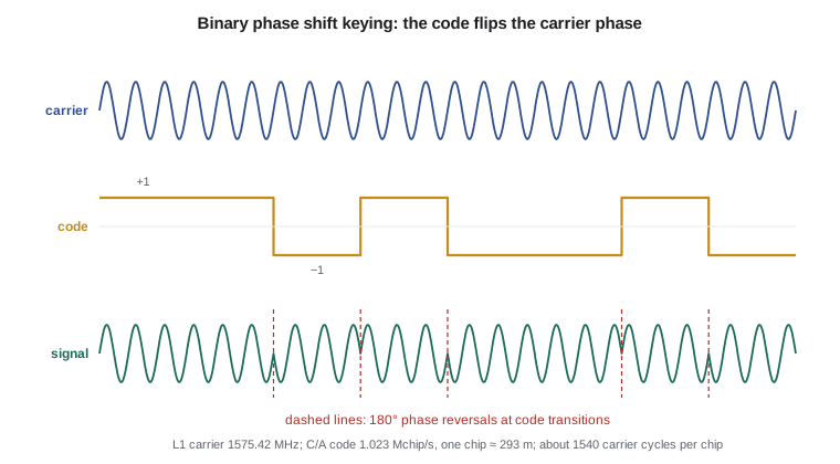
Each GNSS signal is built from three layers. The carrier is a sinusoidal radio wave in the L band, between about 1.1 and 1.6 GHz, chosen because it passes through clouds and rain with little loss and because antennas for it are small. A spreading code, a pseudorandom sequence of +1 and −1 values called chips, is impressed on the carrier by flipping its phase by 180° whenever the code changes sign; this is binary phase shift keying (BPSK). Finally, a slow stream of navigation data, at 50 bits per second for the legacy GPS signal, is added on top of the code. The data carry the satellite's orbit and clock parameters, its health and the time.

The spreading code does two jobs. First, it lets many satellites share one frequency: each satellite has its own code, nearly uncorrelated with the others, and a receiver that correlates the incoming signal with a replica of one satellite's code picks out that satellite alone. This is code division multiple access (CDMA). Second, the code is a ruler. The receiver measures the time offset at which its replica best matches the received code, and that offset, multiplied by the speed of light, is a range measurement. The legacy GPS C/A code has 1023 chips repeated every millisecond, a chip rate of 1.023 MHz, so each chip is about 293 m long; the modern L5 code runs ten times faster, with chips about 29 m long, and gives a sharper correlation peak and better resistance to multipath.

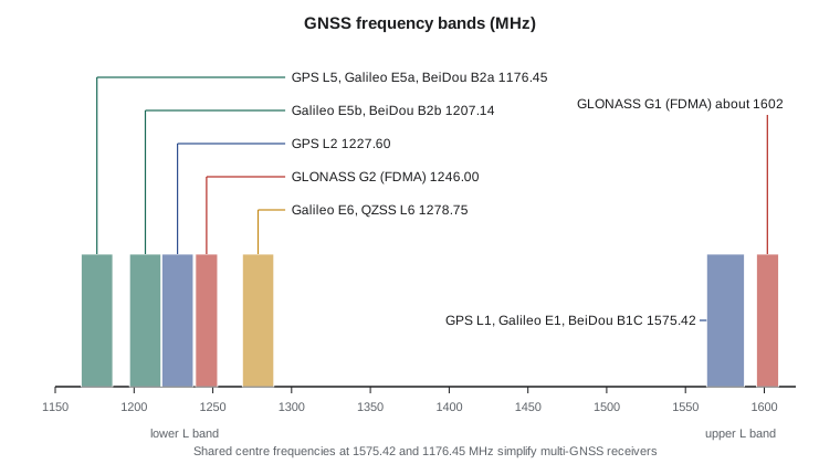
Modern signals refine this design. Most have two components: a data channel carrying the navigation message and a dataless pilot channel that a receiver can track longer and more robustly because no data bits interrupt it. Galileo E1 and GPS L1C use binary offset carrier (BOC) modulations, which split the signal power into two lobes either side of the centre frequency, sharing the band with the legacy C/A signal while improving tracking precision. Galileo E5 is a very wide signal whose two halves, E5a and E5b, can be tracked separately or together as one wideband signal with exceptionally low noise and multipath.

How a receiver tracks a signal

The signal arriving at the antenna is extraordinarily weak, about −128 dBm for the L1 C/A signal, which is roughly 10\(^{-16}\) W and well below the thermal noise in the receiver's bandwidth. It can be recovered only because correlating with the known code over a millisecond or more concentrates its power while the noise averages out. The usual measure of signal quality is the carrier-to-noise density ratio C/N0, expressed in dB-Hz. Open-sky signals at high elevation reach 45 to 50 dB-Hz; values below about 30 dB-Hz indicate obstruction, foliage, interference or a poorly placed antenna, and carrier tracking becomes unreliable.

Inside the receiver, each channel runs two coupled control loops. A delay lock loop keeps the code replica aligned with the incoming code by comparing early and late correlators; its output is the code delay. A phase lock loop keeps a local oscillator aligned with the received carrier, removing the Doppler shift caused by the satellite's motion; its output is the carrier phase and its rate. The Doppler shift for a MEO satellite reaches about ±4 kHz on L1. When the loops hold lock, the receiver records all four observables at each measurement epoch, typically every second for survey work and every 30 s for long static sessions.

The four observables

The pseudorange is the apparent range from satellite to receiver, computed from the measured code delay. It is called pseudo because it is contaminated by the clock errors of both satellite and receiver: a receiver clock error of 1 µs adds about 300 m to every pseudorange. Its precision is typically a few decimetres for the C/A code and a decimetre or better for modern wideband codes, but multipath can add errors of metres. Its great virtue is that it is unambiguous.

The carrier phase is the phase of the received carrier relative to the receiver's oscillator, accumulated since lock was acquired. The receiver measures the fractional cycle at each epoch and counts whole cycles as the range changes. Multiplied by the wavelength, about 19 cm on L1, it is another measure of range, about a hundred times more precise than the code, at the millimetre level. But it is ambiguous: the receiver cannot know how many whole cycles lay between the satellite and the antenna when tracking began. That unknown integer number of cycles, the ambiguity, remains constant as long as tracking continues without interruption. Lessons 7 to 9 are largely about how to determine it.

The Doppler observable is the rate of change of the carrier phase, a measure of the range rate between satellite and receiver; it is used for velocity determination and in cycle slip detection. The fourth observable, C/N0, is not a range at all but is recorded because it describes the quality of the others; it is used for weighting and for detecting interference.

Observation equations

In units of metres, the pseudorange \(P\) and carrier phase \(\Phi\) from satellite \(s\) to receiver \(r\) on frequency \(i\) can be written

where \(\rho\) is the geometric range between the satellite's antenna at transmission and the receiver's antenna at reception, \(dt_r\) and \(dt^s\) are the receiver and satellite clock errors, \(T\) is the tropospheric delay, \(I\) is the ionospheric delay, \(N\) is the integer ambiguity, \(b\) and \(B\) are hardware delays for code and phase, and \(\varepsilon\) collects noise and multipath. Two features of the equations drive the rest of the course. The ionospheric term has opposite signs for code and phase: the ionosphere delays the code (the group delay) and advances the carrier phase by the same amount. And the ionospheric delay depends on frequency, while every other term except the ambiguities and hardware delays does not.

Combinations of frequencies

The first-order ionospheric delay on frequency \(f\) is \(I = 40.3\,\text{TEC}/f^2\), where TEC is the total electron content along the signal path in electrons per square metre. With two frequencies the delay can be eliminated. The ionosphere-free combination of pseudoranges on \(f_1\) and \(f_2\) is

and the same coefficients apply to carrier phase. The price is noise: for L1 and L5 the coefficients are about 2.26 and −1.26, so if both pseudoranges have the same noise the combination has about 2.6 times as much. Other combinations serve other purposes. The geometry-free combination \(P_2 - P_1\) or \(\Phi_1 - \Phi_2\) removes everything except the ionosphere, hardware biases and ambiguities, and is used to monitor the ionosphere and detect cycle slips. The wide-lane combination of phases, \((f_1\Phi_1 - f_2\Phi_2)/(f_1 - f_2)\), behaves like a signal with wavelength \(c/(f_1 - f_2)\), about 86 cm for L1 and L2 and 75 cm for L1 and L5, which makes its ambiguity much easier to resolve. The Melbourne–Wübbena combination subtracts a narrow-lane code combination from the wide-lane phase, cancelling geometry, clocks, troposphere and first-order ionosphere, so that what remains is the wide-lane ambiguity plus noise; it is a standard tool for wide-lane ambiguity resolution and slip detection.

The program below computes the main wavelengths, code chip lengths, combination coefficients and the ionospheric delay on each frequency for a slant TEC of 30 TEC units, a moderate daytime value. It also compares the received signal power with thermal noise to show where the familiar C/N0 values of about 45 dB-Hz come from.

# Carrier wavelengths, code chip lengths and the main linear combinations
c = 299792458.0                     # speed of light, m/s
f0 = 10.23e6                        # GPS fundamental frequency, Hz
bands = {"L1/E1": 154 * f0, "L2": 120 * f0, "L5/E5a": 115 * f0}
for name, f in bands.items():
    print(name.ljust(7), format(f / 1e6, "9.3f"), "MHz  wavelength", format(100 * c / f, "6.2f"), "cm")

chips = {"C/A code (1.023 Mchip/s)": 1.023e6, "L5 code (10.23 Mchip/s)": 10.23e6}
for name, rate in chips.items():
    print(name.ljust(25), "chip length", format(c / rate, "7.2f"), "m")

f1, f2, f5 = bands["L1/E1"], bands["L2"], bands["L5/E5a"]
# Ionosphere-free combination: coefficients that cancel the 1/f^2 delay
a1 = f1 ** 2 / (f1 ** 2 - f5 ** 2); a5 = -f5 ** 2 / (f1 ** 2 - f5 ** 2)
print("ionosphere-free L1/L5 coefficients:", round(a1, 4), round(a5, 4))
# Noise amplification if both pseudoranges have the same noise sigma
print("noise amplification:", round((a1 ** 2 + a5 ** 2) ** 0.5, 2))
# Wide-lane and narrow-lane wavelengths
for (na, fa), (nb, fb) in ((("L1", f1), ("L2", f2)), (("L1", f1), ("L5", f5))):
    print(na + "-" + nb, "wide-lane", format(100 * c / (fa - fb), "6.1f"), "cm   narrow-lane", format(100 * c / (fa + fb), "5.1f"), "cm")

# First-order ionospheric delay for a slant TEC of 30 TECU (1 TECU = 1e16 electrons/m^2)
TEC = 30e16
for name, f in bands.items():
    print("ionospheric delay on", name.ljust(7), format(40.3 * TEC / f ** 2, "5.2f"), "m")

# Signal power: about -128.5 dBm for L1 C/A at the antenna, compared with thermal noise
k = 1.380649e-23; T = 290.0
import math
N0 = 10 * math.log10(k * T * 1000)  # noise density, dBm/Hz
print("thermal noise density:", round(N0, 1), "dBm/Hz; C/N0 for -128.5 dBm:", round(-128.5 - N0, 1), "dB-Hz")

L1/E1    1575.420 MHz  wavelength  19.03 cm
L2       1227.600 MHz  wavelength  24.42 cm
L5/E5a   1176.450 MHz  wavelength  25.48 cm
C/A code (1.023 Mchip/s)  chip length  293.05 m
L5 code (10.23 Mchip/s)   chip length   29.31 m
ionosphere-free L1/L5 coefficients: 2.2606 -1.2606
noise amplification: 2.59
L1-L2 wide-lane   86.2 cm   narrow-lane  10.7 cm
L1-L5 wide-lane   75.1 cm   narrow-lane  10.9 cm
ionospheric delay on L1/E1    4.87 m
ionospheric delay on L2       8.02 m
ionospheric delay on L5/E5a   8.74 m
thermal noise density: -174.0 dBm/Hz; C/N0 for -128.5 dBm: 45.5 dB-Hz

Observation files and signal names

Survey receivers store observations in proprietary formats, which are converted for processing and archiving into RINEX, the Receiver Independent Exchange Format. RINEX 3 and 4 identify each observable by a three-character code: a type letter (C for code, L for phase, D for Doppler, S for signal strength), a frequency band number, and an attribute for the tracking mode or signal component. C1C is the L1 C/A pseudorange, L5Q the phase of the pilot component of L5, C1X the combined data and pilot of a signal. Processing software uses these codes to apply the right biases and antenna corrections, so a RINEX file whose header is wrong, or whose antenna is not described with its standard name, can corrupt a solution silently.

Two pieces of header information deserve special care. The antenna type and radome must use the standard names of the International GNSS Service (IGS) so that the correct phase centre model is applied. The antenna height must be measured to the antenna reference point (ARP), usually the bottom of the mount, and the measurement method stated. A vertical error of 10 mm in an antenna height propagates directly into the coordinates; mistakes of a whole rod section, 0.1 m or more, are among the most common blunders in GNSS surveying.

Phase centres and cycle slips

The point to which a GNSS measurement refers is not a physical point on the antenna. It is the electrical phase centre, whose position relative to the ARP depends on frequency and varies with the elevation and azimuth of the satellite. Calibrations give a phase centre offset (PCO), a mean position typically a few centimetres above the ARP, and phase centre variations (PCV) of a few millimetres as a function of direction. Satellites have their own antenna offsets, which are much larger, up to a few metres from the centre of mass. Precise processing applies both sets of corrections from the IGS antenna file; mixing receivers whose antennas have different, uncalibrated phase centres can bias heights by a centimetre or more.

A cycle slip is a jump in the integer count of carrier cycles, caused when the phase lock loop briefly loses lock, for example as the antenna passes under a branch or a vehicle drives between it and a satellite. After a slip the phase is offset by an unknown integer number of cycles, so the ambiguity has changed. Processing software detects slips by watching combinations that should change smoothly, such as the geometry-free phase, which varies only slowly with the ionosphere, and the Melbourne–Wübbena combination, which should be constant. A detected slip is either repaired by estimating its size or handled by starting a new ambiguity.