Differential GNSS

The irrigation district wanted its new canal gates, culverts and turnouts mapped for its asset database to about half a metre, faster than RTK crews could do it. Grant Okonkwo's crew drove the route with a mapping-grade receiver on a pole, logging features with code-based differential corrections. The data sheet promised sub-metre accuracy with corrections and two to three metres without. Leah Tran asked why a second receiver sitting on a known point, sometimes tens of kilometres away, could remove most of the error. The answer is that most GNSS errors are shared by receivers that are close together, and differential GNSS measures those shared errors at one place and removes them at another.

The principle

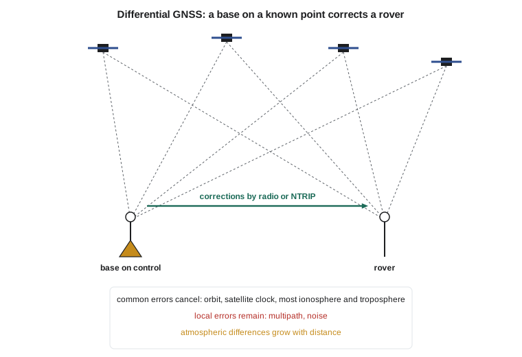
Satellite orbit and clock errors are the same for every user, the ionospheric and tropospheric delays are similar for receivers a few kilometres apart, and even over a hundred kilometres they change smoothly. A base receiver on a point of known coordinates can compute the geometric range to each satellite from its known position and the broadcast orbit, compare it with its measured pseudorange, and attribute the difference to errors. That difference, sent to a nearby rover and applied to the rover's own pseudoranges for the same satellites, removes the common part of the errors. What remains are the errors that differ between the two sites: multipath and receiver noise at each, and the parts of the atmospheric and orbit errors that change with distance.

For satellite \(s\), the pseudorange correction (PRC) at the base \(B\) is

where \(\rho_B^s\) is computed from the known base coordinates and \(dt^s\) is the broadcast satellite clock correction. The rover adds it to its own corrected pseudorange: \(P_R^s + c\,dt^s + \text{PRC}^s\). The base receiver's clock error appears in every correction equally, so it simply adds to the rover's clock error, which the rover estimates anyway. Because corrections change slowly but not negligibly, the base also sends their rate of change, the range rate correction (RRC), so the rover can extrapolate corrections that are a few seconds old.

Range domain and position domain

Corrections can be applied to ranges, as above, or to positions. In the position-domain approach the base computes its own stand-alone position, compares it with its known coordinates and sends the difference. This is simple but works only if the base and rover use exactly the same satellites, because the error in a position depends on which satellites were used. Range-domain corrections let the rover use any subset of the satellites the base corrected, and they are the basis of all standard correction formats.

Delivering corrections

The Radio Technical Commission for Maritime Services Special Committee 104 (RTCM SC-104) defines the standard formats. Version 2 messages carried pseudorange corrections for each satellite; version 3 carries raw observations and, in its multiple signal messages (MSM), code, phase, Doppler and signal strength for every signal of every system, together with base coordinates and antenna information. Corrections reach the rover by UHF or spread-spectrum radio from a local base, by L-band satellite from commercial services, or by the internet using NTRIP (Networked Transport of RTCM via Internet Protocol), in which a caster server relays streams from many bases to rovers that connect through a mobile data link. NTRIP made correction services practical across whole provinces and states and is how most RTK and DGNSS users receive corrections today.

Carrier smoothing

Code multipath and noise at the rover are not removed by differential corrections, and they limit code DGNSS to a few decimetres even with a nearby base. A standard remedy is carrier smoothing with a Hatch filter, which uses the precise change in carrier phase from epoch to epoch to smooth the noisy pseudorange:

with a smoothing window \(n\) of typically 100 s. Because the ionosphere affects code and phase in opposite directions, single-frequency smoothing slowly introduces an error proportional to the change in ionospheric delay over the window, so the window must be limited. Mapping-grade receivers smooth routinely, which is why they typically reach a few decimetres where survey-grade code solutions would be similar and consumer receivers worse.

How the errors decorrelate

The benefit of differential correction depends on the separation between base and rover, and on the age of the corrections. Orbit errors decorrelate as the separation divided by the range to the satellite, so a 1 m orbit error leaves only 5 mm over 100 km. Ionospheric delays decorrelate much faster: on a quiet day the vertical delay changes by a few millimetres per kilometre, and during storms or near the auroral zone by centimetres per kilometre. Tropospheric delays differ with weather and with the height difference between the sites. The program below simulates these effects for eight satellites with typical error sizes and shows how the remaining range error and the horizontal accuracy grow with separation and with the age of corrections.

# Differential GNSS in the range domain: what cancels between a base and a rover
import math, random
random.seed(3)

n_sats = 8
# Errors at the base for each satellite (m): clock, orbit along the line of sight, ionosphere, troposphere
common = [{"clock": random.gauss(0, 1.0), "orbit": random.gauss(0, 0.8),
           "iono": random.uniform(2.0, 6.0), "tropo": random.uniform(2.2, 6.0)} for _ in range(n_sats)]
iono_gradient = 0.004      # m per km of separation, a quiet mid-latitude day
tropo_gradient = 0.001     # m per km, differences in weather and height
orbit_scale = 1 / 20200.0  # orbit error decorrelates roughly as separation / satellite range
local_sigma = 0.25         # carrier-smoothed multipath plus noise at each receiver, not shared

def rover_residuals(d_km, latency_s=0.0, prc_rate_sigma=0.02):
    res = []
    for e in common:
        orbit = e["orbit"] * d_km * orbit_scale                 # what is left of the orbit error
        iono = random.gauss(0, iono_gradient * d_km)
        tropo = random.gauss(0, tropo_gradient * d_km)
        age = random.gauss(0, prc_rate_sigma) * latency_s       # correction grown stale
        local = random.gauss(0, local_sigma) - random.gauss(0, local_sigma)   # base and rover both add their own
        res.append(orbit + iono + tropo + age + local)
    return res

rms = lambda v: math.sqrt(sum(x * x for x in v) / len(v))
standalone = [e["clock"] + e["orbit"] + 0.5 * e["iono"] + 0.05 * e["tropo"] + random.gauss(0, local_sigma) for e in common]
print("stand-alone single-frequency range error RMS:", round(rms(standalone), 2), "m")
HDOP = 0.94
for d in (1, 10, 50, 100, 200, 400):
    trials = [rms(rover_residuals(d)) for _ in range(400)]
    r = sum(trials) / len(trials)
    print("separation", str(d).rjust(3), "km  residual RMS", format(r, "5.2f"), "m  horizontal 95 %", format(2 * HDOP * r, "5.2f"), "m")
for age in (0, 5, 15, 30, 60):
    trials = [rms(rover_residuals(20, age)) for _ in range(400)]
    print("correction age", str(age).rjust(2), "s at 20 km: residual RMS", format(sum(trials) / len(trials), "5.2f"), "m")

stand-alone single-frequency range error RMS: 2.24 m
separation   1 km  residual RMS  0.34 m  horizontal 95 %  0.64 m
separation  10 km  residual RMS  0.34 m  horizontal 95 %  0.64 m
separation  50 km  residual RMS  0.40 m  horizontal 95 %  0.75 m
separation 100 km  residual RMS  0.54 m  horizontal 95 %  1.02 m
separation 200 km  residual RMS  0.87 m  horizontal 95 %  1.64 m
separation 400 km  residual RMS  1.59 m  horizontal 95 %  2.99 m
correction age  0 s at 20 km: residual RMS  0.36 m
correction age  5 s at 20 km: residual RMS  0.36 m
correction age 15 s at 20 km: residual RMS  0.45 m
correction age 30 s at 20 km: residual RMS  0.68 m
correction age 60 s at 20 km: residual RMS  1.21 m

With a nearby base, the residual range error is about 0.34 m, set almost entirely by the multipath and noise at the two receivers, and the horizontal accuracy is about 0.6 m at 95 %, compared with a stand-alone single-frequency range error of 2.2 m. The residual grows slowly to 50 km and then faster: at 400 km it is about 1.6 m, approaching stand-alone performance. Stale corrections also hurt: after 30 s the residual doubles, and after a minute it is worse than at 200 km. Correction services specify a maximum age, often 10 to 30 s, beyond which receivers revert to stand-alone mode.

Satellite-based augmentation: WAAS

A local base serves only users nearby. Wide-area DGNSS uses a network of reference stations spread over a continent to model the errors separately rather than lumping them together, so the corrections are valid everywhere in the network. The Federal Aviation Administration's Wide Area Augmentation System is the North American example. Reference stations across the United States and in Canada and Mexico track the satellites; master stations estimate corrections to each satellite's orbit and clock, a grid of vertical ionospheric delays at points 5° apart, and, critically, bounds on the errors that remain. The corrections and integrity data are uplinked to geostationary satellites and broadcast on the GPS L1 frequency with a GPS-like code, so receivers can use them without extra hardware.

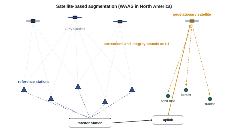
WAAS was designed for aircraft approaches with vertical guidance, such as LPV approaches that guide aircraft down to about 200 ft above the runway without ground-based landing aids. For aviation, the important property is not the typical error but the protection level, a bound on the error that the system guarantees with a very high probability, together with an alert within a few seconds if that guarantee fails. Typical WAAS accuracy is 1 to 2 m horizontally and 2 to 3 m vertically. For surveyors, SBAS is useful for navigation to marks and for GIS work where a metre is acceptable, and its integrity concepts reappear in Lesson 12. Next-generation SBAS will broadcast dual-frequency, multi-constellation corrections on L5, which will remove the ionospheric grid and improve availability.

Canada has no SBAS of its own, but WAAS includes reference stations in Canada and its coverage extends over most of the southern half of the country, including all of Alberta, so Transport Canada has approved WAAS for aviation use. Canada once operated a national wide-area correction service, CDGPS, which was retired in 2011 when commercial and SBAS services covered the need. Coastal radio-beacon DGPS services for marine navigation have also been reduced as SBAS took over their role.

Commercial and precise wide-area services

Several companies operate global correction services delivered by L-band satellites or the internet. Their lower tiers provide decimetre-level wide-area corrections; their higher tiers are precise point positioning services with centimetre accuracy after convergence, discussed in Lesson 9. Galileo's free High Accuracy Service is in the same family. These services estimate orbit and clock corrections for every satellite in real time from a global network, plus, in some cases, regional ionospheric models. The boundaries between DGNSS, SBAS and PPP have become blurred: all of them describe the satellite errors so that a user can remove them, and they differ in how many error sources they model, how precisely, and over what area.

Choosing a method

For Grant's asset mapping, a code-based DGNSS solution from the provincial or state network, or from a commercial service, met the half-metre requirement comfortably with carrier smoothing and a 15° mask. For the canal control, which needed centimetres, it was not adequate, because the residual multipath and noise of code measurements cannot be reduced below a couple of decimetres in a short occupation. That needs carrier phase, which is where the next lesson begins. A good rule is to match the method to the requirement and to the conditions: under trees, near buildings, or with a distant base, code DGNSS degrades gracefully, while carrier-phase methods may fail to fix at all.