Factor models and market efficiency

The CAPM explains expected returns with a single factor, the market. Lesson 6 showed that the evidence points to other sources of risk and return as well. This lesson introduces the arbitrage pricing theory, which allows many factors, and the empirical factor models built from it, especially the Fama–French models now used throughout the industry. It then turns to a closely related question: how efficiently do markets incorporate information? If prices already reflect what is known, analysts cannot expect to beat the market except by taking more risk. The evidence on efficiency, the anomalies that seem to contradict it, and the behavioural explanations offered for them shape how investors should approach active and passive management.

Arbitrage and the arbitrage pricing theory

An arbitrage opportunity is a chance to earn a riskless profit with no net investment, such as buying an asset in one market and selling an identical claim for more in another. In well-functioning markets, such opportunities are rare and fleeting, because traders exploit them until prices line up. Stephen Ross's arbitrage pricing theory (APT), published in 1976, builds an asset pricing model on that one idea instead of on the CAPM's strong assumptions about investor preferences. Suppose returns are driven by a few common factors plus firm-specific noise that diversifies away in large portfolios. Then any well-diversified portfolio's expected return must be a linear function of its sensitivities, or factor betas, to those factors. If it were not, an investor could combine portfolios to cancel all factor risk and still earn a positive return, an arbitrage.

Each \( \lambda \) is the risk premium for one unit of exposure to a factor. The APT does not say what the factors are; that is an empirical question. If the only factor is the market, the APT gives the same answer as the CAPM, but it requires much weaker assumptions: no need for a mean–variance world or for everyone to hold the market portfolio.

Macroeconomic factor models

One way to choose factors is to use surprises in macroeconomic variables that affect many companies' cash flows or discount rates. A classic study by Nai-Fu Chen, Richard Roll and Stephen Ross in 1986 found priced factors for unexpected changes in industrial production, inflation, the spread between low-grade and high-grade bond yields, and the slope of the yield curve. For a Canadian company, sensitivity to commodity prices and the exchange rate with the US dollar is often more important than for a typical US firm, since energy, mining and materials make up a large share of the Canadian market. Macroeconomic models are intuitive but hard to estimate reliably, because the surprises are measured with error.

The Fama–French models

The more popular alternative builds factors from portfolios of shares sorted on characteristics that empirical work has linked to returns. In 1993 Eugene Fama and Kenneth French added two factors to the market: SMB (small minus big), the return on small companies minus large ones, and HML (high minus low), the return on value shares, with high book-to-market ratios, minus growth shares. Mark Carhart added a momentum factor in 1997, the return on recent winners minus recent losers. In 2015 Fama and French extended their model to five factors by adding RMW (robust minus weak profitability) and CMA (conservative minus aggressive investment). Each factor is a long–short portfolio, and an asset's exposure to each is estimated by regressing its excess return on the factor returns.

Whether these factors reflect risk or mispricing is still debated. The risk view says small and value firms are more exposed to hard times, such as financial distress, so investors demand higher returns to hold them. The behavioural view says investors overreact, becoming too pessimistic about value firms and too optimistic about glamorous growth firms. The factors have also been unreliable: the value premium was weak or negative for much of 2007 to 2020, a long drought that tested the patience of value investors.

# Factor regression on seeded simulated monthly data (three-factor model)
import numpy as np
rng = np.random.default_rng(42)
n = 120
mkt = rng.normal(0.006, 0.045, n)
smb = rng.normal(0.003, 0.030, n)
hml = rng.normal(0.004, 0.030, n)
# A fund that looks like it beats the market but simply tilts to small value shares
fund = 0.0 + 1.0 * mkt + 0.5 * smb + 0.6 * hml + rng.normal(0, 0.012, n)

def ols(y, *xs):
    X = np.column_stack([np.ones(len(y)), *xs])
    b, *_ = np.linalg.lstsq(X, y, rcond=None)
    e = y - X @ b
    se = np.sqrt(np.diag(e @ e / (len(y) - X.shape[1]) * np.linalg.inv(X.T @ X)))
    return b, se

b1, se1 = ols(fund, mkt)
b3, se3 = ols(fund, mkt, smb, hml)
print(f"CAPM:         alpha {b1[0] * 12:+.2%} a year (t = {b1[0] / se1[0]:.2f}), beta {b1[1]:.2f}")
print(f"Three-factor: alpha {b3[0] * 12:+.2%} a year (t = {b3[0] / se3[0]:.2f})")
print(f"  loadings: market {b3[1]:.2f}, SMB {b3[2]:.2f}, HML {b3[3]:.2f}")

CAPM:         alpha +6.15% a year (t = 2.29), beta 0.79
Three-factor: alpha +0.45% a year (t = 0.33)
  loadings: market 0.94, SMB 0.48, HML 0.56

The simulated fund has no true skill at all: its returns are just market exposure plus tilts toward small and value shares. Measured against the CAPM, it appears to earn an alpha of about 6 % a year with a t-statistic above 2, because its tilts happened to pay off in this sample. Measured against the three-factor model, the alpha shrinks toward zero and is not statistically significant. That is why the choice of benchmark matters so much in evaluating managers, as lesson 12 discusses. Exchange-traded funds that deliberately tilt toward such factors, often marketed as smart beta or factor investing, give investors these exposures cheaply, without needing to pay a manager for apparent alpha.

The efficient market hypothesis

A market is informationally efficient if prices fully reflect available information, so that no one can consistently earn abnormal returns, returns above those justified by risk, by trading on that information. Eugene Fama's 1970 survey described three forms. Weak-form efficiency says prices reflect all past price and volume data, so technical analysis, the study of charts and trading patterns, cannot earn abnormal returns. Semi-strong-form efficiency says prices reflect all public information, including financial statements, news and analysts' reports, so fundamental analysis cannot either. Strong-form efficiency says prices reflect even private information held by insiders. Efficiency does not mean prices are always right; it means errors are unpredictable, so no strategy based on available information beats the market after adjusting for risk and costs.

Efficiency creates a paradox noted by Sanford Grossman and Joseph Stiglitz in 1980. If markets were perfectly efficient, no one would be paid to gather information, so no one would, and prices would stop reflecting it. Markets must therefore be efficient enough that most investors cannot beat them, but inefficient enough to reward those who do the work and bear the cost of research. Competition among many skilled analysts is what makes beating the market so hard.

Testing efficiency: event studies

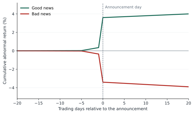
An event study measures how a share's price reacts to news, such as an earnings announcement, merger or dividend change. For each day around the event, the analyst computes the abnormal return: the actual return minus the return predicted by a model such as the market model. Adding up abnormal returns gives the cumulative abnormal return (CAR). In an efficient market, the price should react quickly and fully on the announcement day, with no drift afterward. Studies typically find most of the reaction occurs within minutes or hours of a public announcement, consistent with semi-strong efficiency, though with some exceptions.

Strong-form efficiency is tested by studying insiders. Canadian insiders, such as directors, senior officers and large shareholders, must report trades in their company's securities on the System for Electronic Disclosure by Insiders (SEDI), generally within five days. Trading on material undisclosed information is prohibited under provincial securities law. Studies find that insiders' reported trades earn modest abnormal returns, so markets are not strong-form efficient.

Anomalies

Researchers have documented many patterns that seem to contradict efficiency. Momentum: shares that did well over the past three to twelve months tend to keep doing well for a few more months. Long-term reversal: shares that did very well over three to five years tend to underperform. Post-earnings-announcement drift: prices keep moving in the direction of an earnings surprise for weeks. The value and size effects, and the low-volatility effect from lesson 6. Calendar effects, such as higher returns in January, which have weakened since they became well known. Each anomaly has two possible explanations: it compensates for a risk the model misses, or it reflects mispricing that persists because exploiting it is costly or risky.

Two cautions apply. First, data mining: if thousands of researchers test thousands of strategies on the same data, some will appear profitable by chance. Campbell Harvey and colleagues argued in 2016 that a new factor should clear a much higher statistical bar than the usual t-statistic of 2, perhaps 3 or more. Second, publication: studies find that many anomalies earn much less after they are published, consistent with investors trading them away. Both points suggest that a backtested strategy should be treated with scepticism until it works out of sample.

Behavioural finance

Behavioural finance studies how psychology affects investors and prices. Investors are overconfident, trading too much and underestimating risk; Brad Barber and Terrance Odean found that the households that traded most earned the lowest returns. They show the disposition effect, selling winners too early and holding losers too long. Prospect theory, from Daniel Kahneman and Amos Tversky, describes loss aversion: losses hurt about twice as much as equal gains please. Investors anchor on irrelevant numbers, extrapolate recent trends and follow the crowd. Such biases could be harmless if rational arbitrageurs corrected the prices they distort, but there are limits to arbitrage: exploiting mispricing takes capital, involves risk that the mispricing grows before it shrinks, and may be blocked by short-sale costs. As the saying attributed to John Maynard Keynes puts it, markets can remain irrational longer than a trader can remain solvent.

For most investors, the practical lessons are the same whichever view of markets is right. Beating the market after costs is hard, and most active funds fail to do it consistently, as lesson 12 shows. Diversification, low costs, tax efficiency and avoiding behavioural mistakes are within an investor's control. Those who do pursue active strategies should know what risk factors they are exposed to and whether their edge survives costs and out-of-sample testing.