
FIN-301 · Lesson 5 of 12 · 27 min
Portfolio theory II: the efficient frontier and optimal portfolios
Lesson 4 showed how two risky assets combine and how an investor splits money between a risky portfolio and treasury bills. Real portfolios hold many assets, so this lesson extends the analysis. It shows how to compute the risk of a portfolio of any size, how the efficient frontier is found, why the best risky portfolio is the one where the capital allocation line touches the frontier, and why that leads to the separation of the investment decision into two independent steps. It then turns to the practical problems: the huge number of inputs the method needs, the errors in those inputs, and the shortcuts and constraints professional managers use to cope.
Risk with many assets
With \( n \) assets, the expected return of a portfolio is still the weighted average of the assets' expected returns. Its variance adds up a term for every pair of assets: each asset's own variance weighted by the square of its weight, plus each covariance weighted by the product of the two weights, counted twice. The tidy way to write this uses a vector of weights \( w \) and the covariance matrix \( \Sigma \), whose diagonal holds the variances and whose other entries hold the covariances.
For an equally weighted portfolio of \( n \) assets, the variance simplifies to a striking form. The average variance shrinks with \( 1/n \), while the average covariance remains no matter how many assets are added. As the portfolio grows, its risk falls toward the average covariance between assets, which is the systematic, market-wide risk that diversification cannot remove.
Worked problem
How fast diversification works
Individual shares have an average standard deviation of 40 % and an average correlation of 0.25 with each other. Find the standard deviation of equally weighted portfolios of 1, 10, 30 and very many shares.
Show solution
- Average variance = 0.16; average covariance = 0.25 × 0.16 = 0.04.
- n = 1: σ = 40 %.
- n = 10: variance = 0.016 + 0.9 × 0.04 = 0.052; σ = 22.8 %.
- n = 30: variance = 0.00533 + 0.9667 × 0.04 = 0.04400; σ = 21.0 %.
- Very large n: variance → 0.04; σ → 20 %.
Answer: Most of the benefit comes from the first ten to thirty shares; after that, risk approaches the 20 % floor set by the average covariance.
The efficient frontier
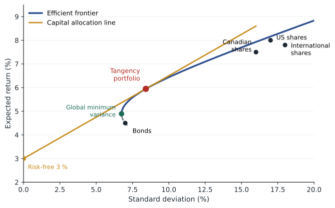
Given expected returns and a covariance matrix for a set of assets, the minimum-variance frontier is the set of portfolios with the lowest variance for each level of expected return. It is found by minimizing \( w^{\top}\Sigma w \) subject to the weights summing to one and the expected return equalling a target, and repeating for many targets. Without restrictions on short selling, the problem has an exact solution using matrix algebra; with restrictions, such as no short positions or maximum weights, it is solved numerically. The upper part of the minimum-variance frontier, above the global minimum-variance portfolio, is the efficient frontier of risky assets. Individual assets typically lie well inside it, because a single asset carries risk that a combination could diversify away.
The optimal risky portfolio and separation
When a risk-free asset is available, every investor can combine it with any risky portfolio along a capital allocation line. The best line is the steepest one, with the highest Sharpe ratio, and it is the line that just touches the efficient frontier. The point of contact is the tangency portfolio, or optimal risky portfolio. Every mean–variance investor, however risk-averse, should hold the risky assets in the same proportions as the tangency portfolio and then use the risk-free asset to set the overall level of risk, as in lesson 4. Without short-sale limits, the tangency weights are proportional to the inverse of the covariance matrix multiplied by the vector of risk premiums.
This result, Tobin's separation property, divides portfolio construction into two independent tasks. The first is technical: estimate the inputs and find the optimal risky portfolio, the same for everyone with the same beliefs. The second is personal: decide how much of it to hold, based on the client's risk aversion, horizon and circumstances. It is the theoretical basis for an industry in which a few funds supply the risky portfolio and advisers tailor the mix of that portfolio and safe assets for each client. It also leads directly to the capital asset pricing model in lesson 6: if everyone holds the same risky portfolio, that portfolio must be the market portfolio.
Worked problem
Building the optimal portfolio of four asset classes
An analyst uses the illustrative assumptions in the code below for Canadian shares, US shares, international shares and bonds, with a risk-free rate of 3 %. Find the global minimum-variance portfolio and the tangency portfolio, with and without allowing short positions.
Show solution
- Form the covariance matrix from the standard deviations and correlations.
- Global minimum variance: w ∝ Σ⁻¹1, scaled to sum to one.
- Tangency without constraints: w ∝ Σ⁻¹(μ − rf), scaled to sum to one.
- With no short sales, search over long-only weights for the highest Sharpe ratio.
Answer: Bonds make up more than half of the tangency portfolio because their low correlation with shares makes them powerful diversifiers. Small changes in expected returns move the weights a lot, which the next sections address.
# Minimum-variance and tangency portfolios for four asset classes (illustrative inputs)
import numpy as np
names = ["Canadian shares", "US shares", "International shares", "Bonds"]
mu = np.array([0.075, 0.080, 0.078, 0.045])
sd = np.array([0.16, 0.17, 0.18, 0.07])
corr = np.array([[1.00, 0.75, 0.70, 0.20],
                 [0.75, 1.00, 0.75, 0.15],
                 [0.70, 0.75, 1.00, 0.15],
                 [0.20, 0.15, 0.15, 1.00]])
cov = np.outer(sd, sd) * corr
rf = 0.03
inv = np.linalg.inv(cov)
ones = np.ones(4)

def stats(w):
    er = w @ mu; vol = np.sqrt(w @ cov @ w)
    return er, vol, (er - rf) / vol

w_gmv = inv @ ones / (ones @ inv @ ones)
w_tan = inv @ (mu - rf); w_tan /= w_tan.sum()

# Long-only tangency by a grid search in steps of 2.5 %
best = None
steps = np.arange(0, 1.0001, 0.025)
for a in steps:
    for b in steps:
        for c in steps:
            d = 1 - a - b - c
            if d < -1e-9: continue
            w = np.array([a, b, c, max(d, 0)])
            s = stats(w)[2]
            if best is None or s > best[0]: best = (s, w)

for label, w in (("global minimum variance", w_gmv), ("tangency, shorts allowed", w_tan), ("tangency, long only", best[1])):
    er, vol, sh = stats(w)
    print(label)
    print("   " + "  ".join(f"{n}: {x:+.1%}" for n, x in zip(names, w)))
    print(f"   E(r) {er:.2%}  sd {vol:.2%}  Sharpe {sh:.3f}")

# Sensitivity: raise the expected return on Canadian shares by half a point
mu2 = mu.copy(); mu2[0] += 0.005
w2 = inv @ (mu2 - rf); w2 /= w2.sum()
print("tangency after +0.5 % on Canadian shares:", " ".join(f"{x:+.1%}" for x in w2))global minimum variance Canadian shares: +3.3% US shares: +5.8% International shares: +2.8% Bonds: +88.2% E(r) 4.89% sd 6.74% Sharpe 0.280 tangency, shorts allowed Canadian shares: +12.9% US shares: +22.2% International shares: +8.6% Bonds: +56.3% E(r) 5.95% sd 8.42% Sharpe 0.350 tangency, long only Canadian shares: +12.5% US shares: +22.5% International shares: +7.5% Bonds: +57.5% E(r) 5.91% sd 8.31% Sharpe 0.350 tangency after +0.5 % on Canadian shares: +24.7% +16.3% +5.2% +53.7%
The output shows the problem every user of mean–variance optimization meets. With these inputs the unconstrained tangency portfolio happens to need no short positions, so it is almost identical to the long-only search, and its Sharpe ratio is well above that of any single asset class. But raising the Canadian forecast by just half a percentage point nearly doubles the Canadian weight, from about 13 % to about 25 %, at the expense of US and international shares. With more assets and similar correlations, the unconstrained optimizer often takes large long and short positions driven by tiny differences in forecasts. It treats the inputs as exact and exploits their errors, which is why it has been called an error maximizer.
Too many inputs: the single-index model
The full method needs, for \( n \) assets, \( n \) expected returns, \( n \) variances and \( n(n-1)/2 \) covariances. For the roughly 220 shares in the S&P/TSX Composite that is more than 24,000 covariances; for the S&P 500 it is about 125,000. William Sharpe's single-index model cuts the problem down by assuming that shares move together only because they all respond to one common factor, the market. Each share's return is then an alpha, plus a beta times the market's excess return, plus a firm-specific surprise uncorrelated with everything else.
Here \( R \) denotes excess returns over the risk-free rate. The model needs only an alpha, a beta and a firm-specific variance for each share, plus the market's expected return and variance: \( 3n + 2 \) estimates instead of \( n(n+3)/2 \). It also splits each share's risk into a systematic part, \( \beta^{2}\sigma_M^{2} \), and a firm-specific part that diversifies away, which is the decomposition behind FIN-201 lesson 10. The cost is that it ignores industry and other common effects, which the multifactor models in lesson 7 add back.
| Number of shares | Full covariance model inputs | Single-index model inputs |
|---|---|---|
| 10 | 65 | 32 |
| 50 | 1,325 | 152 |
| 220 | 24,530 | 662 |
| 500 | 125,750 | 1,502 |
Making optimization work in practice
Professional managers use several techniques to tame the optimizer. They add constraints: no short sales, maximum weights per asset or sector, and limits on turnover. They shrink noisy estimates toward simpler targets, for example pulling sample correlations toward their average. The Black–Litterman approach starts from the returns implied by market-capitalization weights, on the logic that the market portfolio is a sensible neutral position, and tilts away only where the manager has a confident view. Some managers avoid return forecasts altogether: the global minimum-variance portfolio needs only the covariance matrix, and risk parity sets weights so each asset class contributes equally to risk, usually with leverage on bonds. Each approach trades theoretical optimality for robustness.
Home bias is a striking departure from diversification. Canada accounts for roughly 3 % of the value of world share markets, yet Canadian investors have traditionally held a much larger share of their equities at home, partly for familiarity, currency and the dividend tax credit, which applies only to Canadian dividends. The Canadian market is also concentrated: financials and energy make up a large part of the S&P/TSX Composite, so a Canada-only portfolio is less diversified by industry than a global one.
Finally, an optimal portfolio drifts as prices change. A 60/40 portfolio left alone after a strong year for shares may become 70/30, with more risk than intended. Rebalancing, either on a calendar or when weights move outside a band, restores the target. It has costs, including trading costs and taxes in taxable accounts, so many investors rebalance with new contributions or within sheltered accounts first.
Common mistakes
MistakeAdding more shares always reduces risk toward zero.
InsteadRisk falls toward the average covariance, the systematic risk that cannot be diversified away.
MistakeThe tangency portfolio is different for each investor.
InsteadWith the same beliefs and a risk-free asset, everyone holds the same risky portfolio; only the amount differs.
MistakeAn optimizer's output is precise because the mathematics is exact.
InsteadIt amplifies estimation errors in the inputs; small changes in forecasts produce large changes in weights.
MistakeThe single-index model assumes shares are uncorrelated.
InsteadIt assumes they are correlated only through the common market factor.
MistakeHolding mostly home-country shares is just as diversified as holding the world.
InsteadHome bias gives up diversification, especially in a small, concentrated market.
Summary and key terms
- Portfolio variance is wᵀΣw; with many assets it approaches the average covariance.
- The efficient frontier is the upper part of the minimum-variance frontier.
- The optimal risky portfolio is the tangency point of the steepest capital allocation line.
- Separation: everyone holds the same risky portfolio and sets risk with the risk-free asset.
- Unconstrained optimization is very sensitive to estimation errors in expected returns.
- The single-index model cuts the inputs from n(n + 3)/2 to 3n + 2 and splits risk into systematic and firm-specific parts.
- Constraints, shrinkage, Black–Litterman and risk parity make optimization more robust; rebalancing keeps the target mix.
- Covariance matrix
- A table of all asset variances and pairwise covariances.
- Minimum-variance frontier
- The portfolios with the lowest variance for each expected return.
- Global minimum-variance portfolio
- The portfolio with the lowest variance of all.
- Tangency portfolio
- The risky portfolio where the capital allocation line touches the efficient frontier.
- Separation property
- The result that portfolio choice splits into choosing the risky portfolio and choosing how much to hold.
- Single-index model
- A model in which assets are correlated only through one common market factor.
- Firm-specific risk
- Risk unique to one company, which diversification removes.
- Black–Litterman model
- An approach that starts from market-implied returns and adjusts for investor views.
- Risk parity
- A strategy that sets weights so each asset class contributes equally to portfolio risk.
- Home bias
- The tendency to hold more domestic assets than diversification would suggest.
Practice problems
Work each problem on paper first, then reveal the answer to check.
Average share variance 0.09, average covariance 0.02. Variance of an equally weighted 20-share portfolio?
Show answer
0.0045 + 0.95 × 0.02 = 0.0235; σ = 15.3 %.
How many covariances does a 100-asset full model need?
Show answer
100 × 99 ÷ 2 = 4,950.
How many estimates does the single-index model need for 100 assets?
Show answer
3 × 100 + 2 = 302.
β = 1.2, σM = 18 %, firm-specific σ = 25 %. Total variance and share that is systematic?
Show answer
Systematic 0.046656; total 0.109156; systematic share 42.7 %.
Two shares have betas 0.8 and 1.3, σM = 20 %. Covariance under the index model?
Show answer
0.8 × 1.3 × 0.04 = 0.0416.
Why do all investors hold the same tangency portfolio in theory?
Show answer
It gives the highest Sharpe ratio; risk preferences are handled by the risk-free asset.
Name two ways managers make optimization more robust.
Show answer
Constraints such as no short sales; shrinkage of estimates; Black–Litterman; minimum variance.
A 60/40 portfolio grows to 68/32 after a strong year for shares. What does rebalancing do?
Show answer
Sells shares and buys bonds to restore 60/40.
Why does home bias cost a Canadian investor more than a US investor?
Show answer
Canada is a small, concentrated share of the world market.
Portfolio task: look up the regional weights of a global equity index fund and compare them with a typical investor's home-country share.
Show answer
Answers vary; note the fund and date.
Lesson quiz · 5 questions
Score 60% or more to complete this lesson.
Create a free account to save your progress, take quizzes and earn a certificate.