Portfolio theory I: risk aversion, diversification and two assets

In 1952 Harry Markowitz showed that investors should judge each asset not by its own risk but by how it changes the risk of the whole portfolio. FIN-201 lesson 10 introduced the result: combining assets that do not move together reduces risk, and the risk that cannot be diversified away, systematic risk, is what earns a premium. This lesson works through the mathematics behind that idea. It starts with how investors trade off risk and return, then shows how to allocate between a risky portfolio and a risk-free asset, and finally how two risky assets combine. Lesson 5 extends the analysis to many assets and to the choice of the best risky portfolio.

Risk aversion and utility

Most investors are risk-averse: offered a risky investment and a certain one with the same expected return, they choose the certain one. They will hold risk only if paid a risk premium. A convenient way to describe this is a utility score that rewards expected return and penalizes variance. The coefficient \( A \) measures the investor's risk aversion: a risk-neutral investor has \( A = 0 \), and higher values mean a stronger dislike of risk. Studies of how investors actually behave suggest values of roughly 2 to 4 for typical investors, though the number varies widely between people and over a person's life.

Returns and standard deviations in this formula are written as decimals. The certainty equivalent of an investment is the risk-free return that would give the same utility. An investor with \( A = 4 \) looking at a portfolio with an expected return of 8 % and a standard deviation of 20 % has a utility of 0.08 − 0.5 × 4 × 0.04 = 0, so they would be indifferent between that portfolio and a guaranteed return of zero. They would prefer even a 1 % treasury bill. A less risk-averse investor with \( A = 2 \) values the same portfolio at 4 %, and would choose it over the bill.

Investment dealers and advisers in Canada must collect know-your-client information, including the client's risk tolerance, risk capacity, time horizon and investment objectives, and must put the client's interest first when making suitability determinations under the client-focused reforms in force since 2021. Risk questionnaires are a practical, if imperfect, way to estimate a client's risk aversion.

Allocating between a risky portfolio and a risk-free asset

The simplest portfolio decision is how much to put into a diversified risky portfolio \( P \) and how much into a risk-free asset such as treasury bills. If a fraction \( y \) goes into the risky portfolio, the complete portfolio has an expected return that rises in a straight line with \( y \), and a standard deviation equal to \( y \) times the risky portfolio's, because the risk-free asset has no variance and no covariance with anything. Plotting all the combinations gives a straight line from the risk-free rate through the risky portfolio: the capital allocation line (CAL). Points beyond \( P \) represent borrowing at the risk-free rate to invest more than 100 % in the risky portfolio.

The slope of the CAL is the reward-to-volatility ratio, or Sharpe ratio, of the risky portfolio: the extra expected return for each extra unit of standard deviation. Every investor faces the same line if they can invest in the same risky portfolio; what differs is where on the line each chooses to be. Maximizing utility gives the optimal fraction in the risky portfolio.

Covariance and correlation

When two risky assets are combined, what matters is not only their individual risks but how they move together. Covariance measures whether two returns tend to be above or below their averages at the same time. Its size depends on the units, so it is usually scaled into the correlation coefficient, which runs from −1 (perfect opposite movement) through 0 (no linear relationship) to +1 (perfect movement together). Correlations between broad share markets are often 0.6 to 0.9, between shares and high-quality government bonds historically near zero or negative, though that relationship turned positive in 2022, when rising inflation hurt both together.

The two-asset portfolio

A portfolio with weight \( w \) in asset 1 and \( 1 - w \) in asset 2 has an expected return equal to the weighted average of the two expected returns. Its variance is not a simple average: it includes a term for the covariance. That covariance term is where diversification comes from. Unless the correlation is exactly +1, the portfolio's standard deviation is less than the weighted average of the two standard deviations.

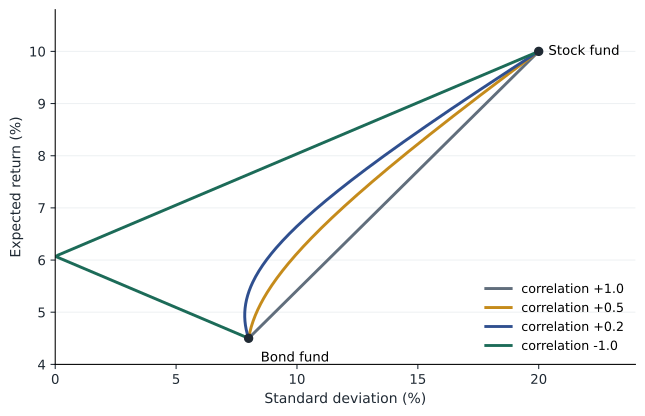
Three cases show the effect of correlation. With \( \rho = +1 \), the portfolio's standard deviation is the weighted average, so there is no diversification benefit; the combinations lie on a straight line. With \( \rho = -1 \), the two assets can be combined to eliminate risk entirely. In between, which is the normal case, the combinations trace a curve that bows to the left: some portfolios have less risk than either asset alone. The weight that gives the minimum-variance portfolio has a closed form.

# Two-asset portfolios: return and risk as the weight and correlation change
import math
er1, sd1 = 0.10, 0.20     # stock fund
er2, sd2 = 0.045, 0.08    # bond fund

def port(w, rho):
    er = w * er1 + (1 - w) * er2
    var = w**2 * sd1**2 + (1 - w)**2 * sd2**2 + 2 * w * (1 - w) * rho * sd1 * sd2
    return er, math.sqrt(var)

def w_min(rho):
    cov = rho * sd1 * sd2
    return (sd2**2 - cov) / (sd1**2 + sd2**2 - 2 * cov)

for rho in (1.0, 0.5, 0.2, 0.0, -0.5, -1.0):
    w = w_min(rho)
    er, sd = port(w, rho)
    print(f"rho {rho:+.1f}: min-variance weight in stocks {w:6.3f}  E(r) {er:6.2%}  sd {sd:6.2%}")
print()
for w in (0.0, 0.2, 0.4, 0.6, 0.8, 1.0):
    er, sd = port(w, 0.2)
    print(f"w = {w:.1f}: E(r) {er:.2%}  sd {sd:.2%}")

rho +1.0: min-variance weight in stocks -0.667  E(r)  0.83%  sd  0.00%
rho +0.5: min-variance weight in stocks -0.053  E(r)  4.21%  sd  7.95%
rho +0.2: min-variance weight in stocks  0.080  E(r)  4.94%  sd  7.84%
rho +0.0: min-variance weight in stocks  0.138  E(r)  5.26%  sd  7.43%
rho -0.5: min-variance weight in stocks  0.231  E(r)  5.77%  sd  5.55%
rho -1.0: min-variance weight in stocks  0.286  E(r)  6.07%  sd  0.00%

w = 0.0: E(r) 4.50%  sd 8.00%
w = 0.2: E(r) 5.60%  sd 8.20%
w = 0.4: E(r) 6.70%  sd 10.12%
w = 0.6: E(r) 7.80%  sd 13.02%
w = 0.8: E(r) 8.90%  sd 16.40%
w = 1.0: E(r) 10.00%  sd 20.00%

With a correlation of +1, the formula gives a negative weight: it shorts two-thirds of a unit of the stock fund for every unit of portfolio and puts 1.67 units in bonds, which removes all risk but leaves an expected return of only 0.83 %. Without short selling, perfectly correlated assets offer no diversification at all. At a correlation of −1, zero risk is reached with positive weights in both funds. Real assets lie in between, which is why diversification reduces risk but cannot eliminate it.

From two assets to the efficient set

The curve of two-asset portfolios has two parts. Portfolios on the upper part, above the minimum-variance point, offer the highest expected return for their level of risk and are called efficient. Portfolios on the lower part are dominated: another portfolio has the same risk and a higher return. No rational risk-averse investor would hold a dominated portfolio. With many assets, as lesson 5 shows, the same logic produces the efficient frontier, and adding a risk-free asset turns the investor's problem into choosing the single risky portfolio that gives the steepest capital allocation line.

Two practical points temper the theory. First, the inputs, expected returns, standard deviations and especially correlations, are estimated from limited and noisy data and change over time; correlations tend to rise in crises, exactly when diversification is most needed. Second, investors care about more than mean and variance, including liquidity, taxes, ethics and the fat tails described in lesson 3. Portfolio theory is a disciplined starting point, not a machine that produces the right answer.