Measuring return and risk

Before an investor can choose between investments, they need a consistent way to measure what each has earned and how risky it has been. FIN-201 lesson 10 introduced holding-period returns, the arithmetic and geometric averages, and the standard deviation as a measure of total risk. This lesson builds the toolkit an investment professional uses: returns measured over different periods and with cash flows in and out, real and continuously compounded returns, expected returns from scenarios, the shape of return distributions, and downside measures such as value at risk, expected shortfall and drawdown. These measures recur in every later lesson, from portfolio construction to performance evaluation.

Holding-period and annualized returns

The holding-period return (HPR) over any interval is the ending value plus income received, divided by the beginning value, minus one. Returns over different lengths of time cannot be compared until they are put on a common basis, usually a year. A return earned over a fraction of a year is annualized by compounding: a 2 % return over three months is equivalent to an effective annual return of 1.02⁴ − 1 = 8.24 %. Returns over several years are annualized with the geometric mean. Annualizing a short-term return assumes it could be repeated, which is rarely true, so very short-period annualized figures, such as a fund's best month, should be treated with suspicion.

Here \( T \) is the length of the period in years. For a three-month return, \( T = 0.25 \), so the exponent is 4.

When returns are added across periods, as in some statistical work, investors often use continuously compounded, or log, returns: the natural logarithm of one plus the simple return. Log returns add over time, so the log return over a year is the sum of the monthly log returns, and they suit models like Black–Scholes in lesson 11. For small returns, simple and log returns are nearly the same; for large ones they differ noticeably, and a loss of 50 % in log terms is −69.3 %.

Arithmetic versus geometric averages

The arithmetic average of a series of returns is the best estimate of the expected return for a single future period. The geometric average is the constant rate that would have produced the same ending wealth, so it describes what an investor actually experienced over several periods. The geometric average is always lower than the arithmetic when returns vary, and the gap grows with volatility; roughly, the geometric mean is about the arithmetic mean minus half the variance. A fund that gains 50 % one year and loses 50 % the next has an arithmetic average of 0 % but has lost a quarter of its value; its geometric average is −13.4 %. Fund marketing often quotes whichever figure looks better, so the reader should always ask which average is being shown.

Money-weighted and time-weighted returns

When money flows into or out of a portfolio, there are two ways to measure performance. The money-weighted return is the internal rate of return of the investor's cash flows: deposits, withdrawals and the ending value. It measures the investor's own experience, including the effect of when they added or removed money. The time-weighted return links the returns of each sub-period between cash flows, removing the effect of the flows. It measures the manager's skill, since managers do not control when clients add or withdraw money, and it is the standard required by the Global Investment Performance Standards (GIPS) for reporting fund performance.

Since 2016, Canadian investment dealers have been required by the client relationship model, phase 2 (CRM2) rules to send clients an annual performance report showing money-weighted returns, along with the dollar amount of fees and charges paid. Fund documents, by contrast, report time-weighted returns.

Real returns

Nominal returns are measured in dollars; real returns measure the change in purchasing power. The exact relationship, from the Fisher equation in ECON-102 lesson 6, is that one plus the real return equals one plus the nominal return divided by one plus the inflation rate. The common shortcut, nominal minus inflation, is close when rates are low but overstates the real return when inflation is high. Inflation matters most for long-term investors: at 3 % inflation, a dollar loses about 45 % of its purchasing power in 20 years. That is why treasury bills, though nearly riskless in nominal terms, can be risky in real terms, and why inflation-indexed bonds, discussed in lesson 9, appeal to retirement savers.

Expected return and variance from scenarios

Looking forward, an analyst may describe an investment by a set of scenarios with probabilities. The expected return is the probability-weighted average of the scenario returns, and the variance is the probability-weighted average of squared deviations from the expected return. The standard deviation is the square root of the variance. This is the same calculation used for historical data, except that probabilities replace equal weights. Scenario analysis makes the analyst's assumptions explicit, which is useful even though the probabilities are subjective.

The shape of return distributions

Much of finance assumes returns follow a normal distribution, which is fully described by its mean and standard deviation. Under that assumption, returns fall within one standard deviation of the mean about two-thirds of the time and within two standard deviations about 95 % of the time. Real returns depart from the normal in two important ways. They are often negatively skewed, with occasional large losses and fewer large gains, and they have fat tails, or excess kurtosis, so extreme moves happen far more often than the normal distribution predicts. The October 1987 crash, when North American markets fell more than 20 % in a day, would be essentially impossible under a normal distribution fitted to earlier data. Investors who rely only on the standard deviation will understate the risk of disaster.

Value at risk, expected shortfall and drawdown

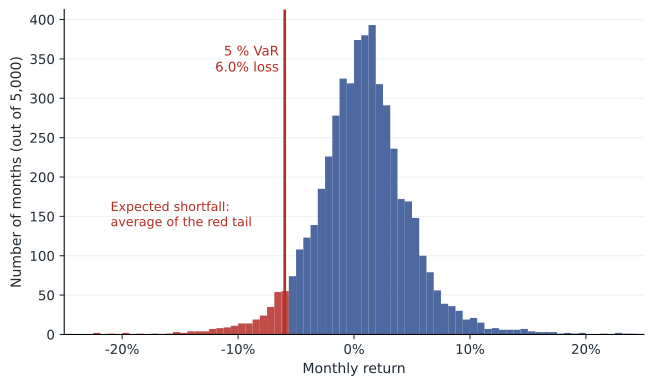
Value at risk (VaR) answers a specific question: what loss will be exceeded only with a given small probability over a given period? A one-month 5 % VaR of 8 % means there is a 5 % chance of losing more than 8 % in a month. Historical VaR reads the cut-off directly from past or simulated returns; parametric VaR assumes a normal distribution and uses the mean minus 1.645 standard deviations for the 5 % level. VaR says nothing about how bad losses can be beyond the cut-off, so regulators and risk managers increasingly use expected shortfall (also called conditional VaR), the average loss in the worst 5 % of cases. Banks' trading-book capital rules under the Basel framework moved from VaR to expected shortfall for this reason.

Long-term investors also watch the maximum drawdown: the largest fall from a previous peak to a subsequent trough. Drawdowns capture what investors actually feel, because a portfolio that loses 40 % needs a 67 % gain to recover. Broad share indices in both countries fell roughly half from peak to trough in 2008–2009, and recovering took several years.

# Risk measures on seeded simulated monthly returns with fat tails
import math
import numpy as np
rng = np.random.default_rng(301)
n = 5000
# Student t with 4 degrees of freedom, scaled to a 4.5 % monthly standard deviation
t = rng.standard_t(4, n)
r = 0.007 + 0.045 * t / np.sqrt(4 / (4 - 2))

mean, sd = r.mean(), r.std(ddof=1)
skew = ((r - mean) ** 3).mean() / sd ** 3
kurt = ((r - mean) ** 4).mean() / sd ** 4 - 3
hist_var = -np.percentile(r, 5)
param_var = -(mean - 1.645 * sd)
es = -r[r <= np.percentile(r, 5)].mean()
print(f"mean {mean:.2%}  sd {sd:.2%}  skew {skew:.2f}  excess kurtosis {kurt:.2f}")
print(f"5 % VaR: historical {hist_var:.2%}, normal {param_var:.2%}")
print(f"expected shortfall {es:.2%}")
print(f"months worse than -15 %: {np.sum(r < -0.15)} (normal model predicts about {n * 0.5 * (1 + math.erf((-0.15 - mean) / (sd * math.sqrt(2)))):.1f})")

# Maximum drawdown on the first 240 months
wealth = np.cumprod(1 + r[:240])
peak = np.maximum.accumulate(wealth)
print(f"maximum drawdown over 20 years: {(wealth / peak - 1).min():.1%}")

mean 0.71%  sd 4.36%  skew -0.02  excess kurtosis 6.00
5 % VaR: historical 5.98%, normal 6.47%
expected shortfall 9.11%
months worse than -15 %: 15 (normal model predicts about 0.8)
maximum drawdown over 20 years: -32.6%

The simulated returns show the fat-tail effect clearly. The 5 % VaR from the simulated data is actually a little smaller than the normal estimate, yet the normal model predicts fewer than one month worse than −15 % where the simulation produced 15. Fat tails hide beyond the VaR cut-off, which is exactly why expected shortfall is worth reporting. (This simulation is symmetric, so it shows fat tails but not the negative skew of real markets.) In practice, analysts compare several measures and run stress tests based on historical crises rather than trusting any single number.

Risk-adjusted return: a first look

A return alone says little without the risk taken to earn it. The simplest risk-adjusted measure is the Sharpe ratio: the excess return over the risk-free rate divided by the standard deviation. It measures the reward per unit of total risk and reappears in lesson 5 as the slope of the capital allocation line and in lesson 12 as a performance measure. A portfolio with a 9 % return, a 3 % risk-free rate and a 15 % standard deviation has a Sharpe ratio of 0.40. Like all historical measures, the Sharpe ratio depends heavily on the period chosen, and it treats upside and downside volatility the same, which is why some analysts prefer the Sortino ratio, which uses only downside deviation.