
FIN-201 · Lesson 9 of 12 · 34 min
Risk analysis in capital budgeting
A project's NPV is calculated from forecasts, and every forecast is uncertain. Sales may fall short, costs may rise, a competitor may cut prices, a regulation may change. The discount rate, developed in lessons 10 and 11, compensates investors for the kind of risk that cannot be diversified away. But managers also need to understand the project's own risks: which assumptions drive the result, how bad things could get, and what they can do if events turn out differently. This lesson covers the main tools: sensitivity analysis, scenario analysis, break-even analysis, operating leverage, Monte Carlo simulation, decision trees and real options. None of them replaces NPV; each helps decide how much to trust it.
The base case
Throughout this lesson we use one project. It requires an investment of $2.0 million, lasts five years and has no salvage value. The firm expects to sell 40,000 units a year at $60 each, with variable costs of $35 a unit and fixed cash costs of $300,000 a year. To keep the arithmetic transparent, assume the investment is deducted for tax in equal amounts of $400,000 a year over five years (lesson 8 showed how the actual Canadian and US rules differ). The tax rate is 25 % and the discount rate 11 %.
Worked problem
Base-case NPV
Find the annual operating cash flow and NPV of the project in its base case.
Show solution
- Contribution = 40,000 × (60 − 35) = 1,000,000; minus fixed costs 300,000 gives 700,000 before tax.
- After-tax operating cash flow = 700,000 × 0.75 + 400,000 × 0.25 = 525,000 + 100,000 = 625,000.
- Annuity factor at 11 % for 5 years = 3.69590.
- NPV = −2,000,000 + 625,000 × 3.69590 = 309,936.
Answer: In the base case the project adds about $310,000 of value. The question is how confident the firm can be in that figure.
Sensitivity analysis
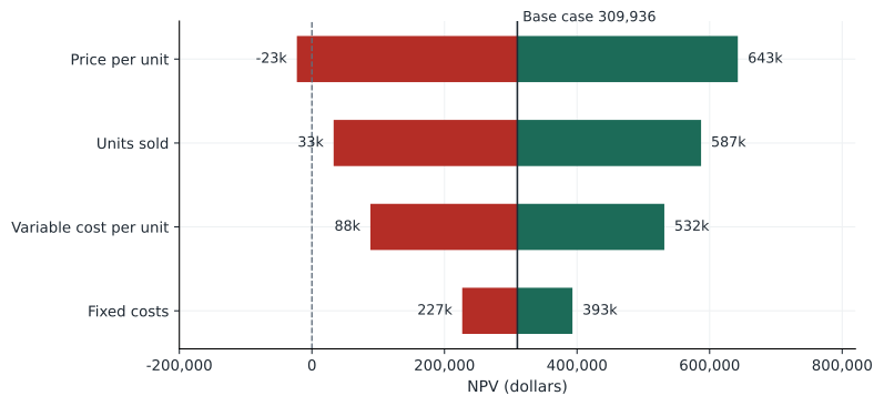
Sensitivity analysis changes one input at a time, holding the others at their base-case values, and records how NPV responds. It shows which variables matter most, and therefore where better information or tighter management is most valuable. Results are often shown as a tornado chart, with the variables sorted by the width of their NPV range. The weakness of sensitivity analysis is that variables rarely move one at a time: in a recession, volumes and prices may fall together. And the ranges used must be realistic; a variable looks important simply if it is given a wide range.
| Variable | Low value | NPV at low | High value | NPV at high |
|---|---|---|---|---|
| Units sold | 36,000 | 32,743 | 44,000 | 587,128 |
| Price per unit | $57 | −22,695 | $63 | 642,566 |
| Variable cost per unit | $37 | 88,182 | $33 | 531,689 |
| Fixed costs | $330,000 | 226,778 | $270,000 | 393,093 |
Scenario analysis
Scenario analysis changes several variables together in a consistent story. A pessimistic scenario might combine lower volume, lower price, higher unit costs and higher fixed costs, as might happen if a strong competitor entered; an optimistic one the reverse. Scenarios capture the correlation between variables that sensitivity analysis ignores, and they force managers to think through how the business would actually behave. Their weakness is that they give only a few points, with no measure of how likely each is.
Worked problem
Three scenarios
In the pessimistic scenario the firm sells 32,000 units at $56, with variable costs of $37 and fixed costs of $330,000. In the optimistic scenario it sells 46,000 units at $63, with variable costs of $33 and fixed costs of $280,000. Find the NPV in each.
Show solution
- Pessimistic: pre-tax = 32,000 × 19 − 330,000 = 278,000; OCF = 208,500 + 100,000 = 308,500; NPV = −2,000,000 + 308,500 × 3.6959 = −859,816.
- Optimistic: pre-tax = 46,000 × 30 − 280,000 = 1,100,000; OCF = 825,000 + 100,000 = 925,000; NPV = 1,418,705.
- Base case: 309,936.
Answer: The range from −$0.86 million to +$1.42 million is wide. Whether the project is acceptable depends on how likely the pessimistic case is and whether the firm can limit its losses if it happens.
Break-even analysis
Break-even analysis asks how low sales can fall before the project stops paying its way. The accounting break-even is the volume at which accounting profit is zero: fixed costs plus depreciation, divided by the contribution margin per unit. It is a misleading target, because a project that only breaks even in accounting terms loses money in present value: it returns the original investment with no return on it. The NPV break-even, also called financial break-even, is the volume at which NPV is zero. It requires the operating cash flow to cover the equivalent annual cost of the investment.
Worked problem
Accounting and NPV break-even
Find the accounting and NPV break-even volumes for the project.
Show solution
- Accounting: (300,000 + 400,000) ÷ 25 = 28,000 units a year.
- Equivalent annual cost of the investment = 2,000,000 ÷ 3.6959 = 541,141.
- Set (25Q − 300,000) × 0.75 + 100,000 = 541,141, so 25Q − 300,000 = 588,188 and Q = 35,528 units.
Answer: The project must sell about 35,500 units a year to earn its cost of capital, 27 % more than the accounting break-even and only about 11 % below the base case.
Operating leverage
Projects with high fixed costs and low variable costs are more sensitive to volume than projects with the opposite structure. The degree of operating leverage (DOL) measures this: the percentage change in operating profit for a 1 % change in sales volume. A highly automated plant has high operating leverage: profits soar when volume is strong and collapse when it is weak. Choosing a cost structure, for example whether to automate, outsource or lease, is therefore partly a choice about risk.
Worked problem
Degree of operating leverage
Find the project's DOL at the base case, counting the $400,000 tax deduction as a fixed cost, and interpret it.
Show solution
- Contribution = 1,000,000; EBIT = 1,000,000 − 300,000 − 400,000 = 300,000.
- DOL = 1,000,000 ÷ 300,000 = 3.33.
Answer: A 10 % fall in volume cuts operating profit (EBIT) by about 33 %. That high leverage explains why volume appears so prominently in the sensitivity analysis.
Monte Carlo simulation
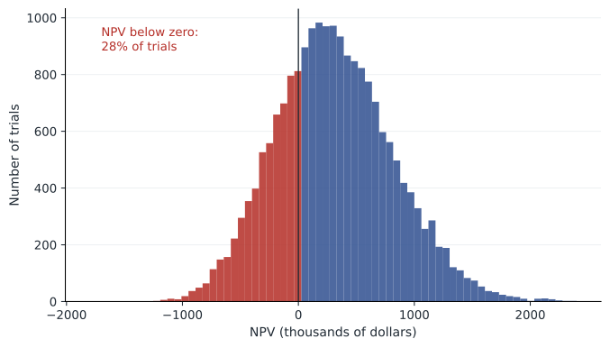
Monte Carlo simulation extends scenario analysis to thousands of scenarios. The analyst specifies a probability distribution for each uncertain input, and correlations between them where relevant; the computer draws random values, calculates the NPV for each draw, and builds a distribution of outcomes. The result shows the expected NPV, the spread of outcomes and the probability of a negative NPV. Simulation is widely used in mining, energy, pharmaceuticals and real estate. Two cautions apply. First, the output is only as good as the input distributions, which are often guesses. Second, the distribution of NPV is not a reason to change the discount rate or to reject a project just because it might lose money: investors care about systematic risk, which the discount rate already reflects, while the spread of a single project's NPV mostly reflects risk that diversified shareholders can avoid.
# Monte Carlo simulation of the project's NPV
import random, statistics
random.seed(201)
annuity = (1 - 1.11 ** -5) / 0.11
def npv(units, price, var_cost, fixed):
    ocf = (units * (price - var_cost) - fixed) * 0.75 + 400_000 * 0.25
    return -2_000_000 + ocf * annuity

results = []
for _ in range(20_000):
    units = random.gauss(40_000, 5_000)
    price = random.gauss(60, 3)
    var_cost = random.gauss(35, 1.5)
    fixed = random.uniform(280_000, 320_000)
    results.append(npv(units, price, var_cost, fixed))
results.sort()
print(f"mean NPV {statistics.mean(results):,.0f}")
print(f"standard deviation {statistics.stdev(results):,.0f}")
print(f"5th percentile {results[1000]:,.0f}   95th percentile {results[19000]:,.0f}")
print(f"probability NPV < 0: {sum(v < 0 for v in results) / len(results):.1%}")mean NPV 310,134 standard deviation 508,804 5th percentile -487,409 95th percentile 1,184,340 probability NPV < 0: 27.9%
Decision trees
Many projects are not all-or-nothing commitments made once. Managers can gather information, wait, expand, scale back or abandon as events unfold. A decision tree maps out the sequence of decisions and uncertain events, with probabilities and cash flows, and is solved backwards: at each decision point, choose the branch with the highest value; at each chance point, take the probability-weighted average; discount back to the present.
Worked problem
Test-marketing before launch
Instead of launching now, the firm can spend $100,000 on a one-year test market. With probability 0.6 the test is favourable and a launch next year would then have an NPV (at that date) of $950,000; with probability 0.4 it is unfavourable and a launch would have an NPV of −$650,000, so the firm would not launch. The expected NPV of launching now is the base case, about $310,000. Should the firm test first?
Show solution
- Launch now: expected NPV = 0.6 × 950,000 + 0.4 × (−650,000) = 310,000 (consistent with the base case).
- Test first: after a favourable test, launch (950,000); after an unfavourable one, stop (0).
- Value of testing = −100,000 + (0.6 × 950,000 + 0.4 × 0) ÷ 1.11 = −100,000 + 513,514 = 413,514.
Answer: Testing first is worth about $103,500 more than launching now, because it lets the firm avoid the bad outcome. The value comes from the option to walk away, not from the test itself.
Real options
The test-market example shows a general point: flexibility has value. Opportunities to change course after information arrives are called real options, by analogy with financial options. The main types are the option to expand if a project does well, the option to abandon and recover salvage value if it does badly, the option to delay until uncertainty is resolved, and the option to switch inputs, outputs or locations. A standard NPV calculation that assumes the firm will follow a fixed plan whatever happens undervalues projects with such options. Real options also explain some apparently odd behaviour, such as a firm investing in a small, negative-NPV pilot project because it opens the door to a large follow-on investment.
Worked problem
An abandonment option
A year from now the project will be worth either $2.6 million or $1.0 million (present value of its remaining cash flows at that date), each with probability 0.5. The equipment could then be sold for $1.4 million. The discount rate is 11 %. What is the abandonment option worth?
Show solution
- Without the option: value today = (0.5 × 2.6 + 0.5 × 1.0) ÷ 1.11 = 1.6216 million.
- With the option, the firm sells if the value is 1.0 million: (0.5 × 2.6 + 0.5 × 1.4) ÷ 1.11 = 1.8018 million.
- Value of the option = 1.8018 − 1.6216 = 0.1802 million.
Answer: The right to abandon adds about $180,000. Discounting option payoffs at the project's cost of capital is a simplification; option pricing methods covered in FIN-301 handle the changing risk more precisely.
Managing forecast risk
Formal risk analysis cannot fix biased forecasts. Studies of large projects, such as Bent Flyvbjerg's research on infrastructure, find systematic cost overruns and benefit shortfalls, driven by optimism and by incentives to get projects approved. Practical safeguards include asking where the project's positive NPV comes from (what advantage lets the firm earn more than competitors?), comparing forecasts with a reference class of similar past projects, separating the people who propose projects from those who review them, and conducting post-completion audits. CON-310 and PMP courses discuss the management side of keeping projects on budget.
Common mistakes
MistakeA project that breaks even in accounting terms is acceptable.
InsteadAccounting break-even ignores the return on capital; use the NPV break-even.
MistakeSensitivity analysis shows the realistic range of outcomes.
InsteadIt moves one variable at a time; scenarios and simulation capture joint movements.
MistakeA high probability of a negative NPV means the discount rate should be raised.
InsteadThe discount rate reflects systematic risk; project-specific spread is mostly diversifiable.
MistakeNPV assumes managers cannot change plans.
InsteadStandard NPV often ignores flexibility; real options add the value of adapting.
MistakeMonte Carlo output is precise because it uses thousands of trials.
InsteadIt is only as reliable as the input distributions and correlations.
Summary and key terms
- Sensitivity analysis changes one input at a time and identifies critical variables; a tornado chart ranks them.
- Scenario analysis changes inputs together in consistent stories.
- Accounting break-even = (F + D) ÷ (P − V); NPV break-even requires operating cash flow to cover the equivalent annual cost of the investment.
- Operating leverage magnifies the effect of volume on operating profit.
- Monte Carlo simulation produces a distribution of NPVs from input distributions.
- Decision trees value sequential decisions by working backwards.
- Real options to expand, abandon, delay or switch add value that a static NPV misses.
- Sensitivity analysis
- Analysis of how NPV changes when one input is varied.
- Tornado chart
- A chart ranking inputs by the size of their effect on NPV.
- Scenario analysis
- Analysis of NPV under consistent combinations of input values.
- Accounting break-even
- The volume at which accounting profit is zero.
- NPV break-even
- The volume at which a project's NPV is zero.
- Degree of operating leverage
- The percentage change in operating profit for a 1 % change in sales volume.
- Monte Carlo simulation
- Repeated random sampling of inputs to build a distribution of outcomes.
- Decision tree
- A diagram of sequential decisions and chance events solved backwards.
- Real option
- The right, but not the obligation, to change a project's course as information arrives.
- Abandonment option
- The right to stop a project and recover its salvage value.
Practice problems
Work each problem on paper first, then reveal the answer to check.
Price $40, variable cost $24, fixed costs $200,000, annual depreciation $120,000. Accounting break-even?
Show answer
320,000 ÷ 16 = 20,000 units.
An investment of $1 million over 4 years at 10 %. Equivalent annual cost?
Show answer
1,000,000 ÷ 3.1699 = 315,471.
Why is NPV break-even higher than accounting break-even?
Show answer
It requires a return on the invested capital, not just its recovery.
Contribution 800,000, fixed costs and depreciation 600,000. DOL?
Show answer
800 ÷ 200 = 4.
With DOL 4, sales volume falls 5 %. Change in EBIT?
Show answer
About −20 %.
Name a weakness of sensitivity analysis.
Show answer
It ignores correlations between variables, and results depend on chosen ranges.
A test costing $50,000 now reveals success (p = 0.5, NPV next year 600,000) or failure (stop). r = 10 %. Value of testing?
Show answer
−50,000 + 300,000 ÷ 1.1 = 222,727.
A project is worth 3.0 or 1.2 million next year (equal chances); it can be sold for 1.8 million. r = 10 %. Value of the abandonment option?
Show answer
(0.5 × 0.6) ÷ 1.1 = 0.273 million.
Why might a firm accept a negative-NPV pilot project?
Show answer
It creates an option to make a larger, valuable follow-on investment.
Portfolio task: build a spreadsheet Monte Carlo model of a simple project with at least three uncertain inputs and report the probability of a negative NPV.
Show answer
Answers vary; state distributions and the random seed or number of trials.
Lesson quiz · 5 questions
Score 60% or more to complete this lesson.
Create a free account to save your progress, take quizzes and earn a certificate.