
FIN-201 · Lesson 10 of 12 · 29 min
Risk and return
Investors demand higher returns for bearing more risk; that is why the discount rates in this course depend on the risk of the cash flows. But what kind of risk, and how much extra return? This lesson measures return and risk, looks at what history says about the reward for risk, and explains the most important idea in modern finance: diversification eliminates much of the risk of individual assets, so only the risk that cannot be diversified away earns a reward. That leads to beta and the capital asset pricing model (CAPM), introduced here as the standard tool for estimating the cost of equity in lesson 11. Portfolio theory, factor models and their empirical tests are covered in depth in FIN-301. Nothing in this lesson is a recommendation to buy or sell any investment.
Measuring return
The holding period return on an investment is the income received plus the change in price, divided by the price at the start. For a share, income is the dividend; for a bond, the coupon. Returns over several periods can be averaged in two ways. The arithmetic mean is the simple average of the periodic returns and is the best estimate of the expected return for a single future period. The geometric mean is the constant rate that would produce the same ending wealth, and it is the right measure of past compound growth. The geometric mean is always lower than the arithmetic mean when returns vary, and the gap grows with volatility.
Worked problem
Arithmetic and geometric averages
A share returns +40 %, −20 %, +25 % and −10 % in four successive years. Find the arithmetic and geometric average returns and the ending value of $1,000.
Show solution
- Arithmetic mean = (40 − 20 + 25 − 10) ÷ 4 = 8.75 %.
- Wealth relative = 1.40 × 0.80 × 1.25 × 0.90 = 1.26; $1,000 grows to $1,260.
- Geometric mean = 1.26^(1/4) − 1 = 5.95 %.
Answer: The investor's money actually compounded at 5.95 % a year. The arithmetic mean of 8.75 % is the better forecast for a single year, but overstates multi-year growth.
Measuring risk
Risk in finance means uncertainty about returns. The usual measure for an asset held on its own is the standard deviation of returns, the square root of the variance, which measures how widely returns spread around their mean. With historical data, the sample variance divides the sum of squared deviations by \( n - 1 \). If returns were normally distributed, about two-thirds would fall within one standard deviation of the mean and about 95 % within two. Real returns have fatter tails than the normal distribution, so extreme events such as the 2008 crash or the March 2020 collapse happen more often than the normal curve predicts.
What history shows
Long-run data for many countries show a consistent pattern: shares have earned more than bonds, and bonds more than treasury bills, but with much greater year-to-year swings. Studies such as the Dimson, Marsh and Staunton global returns data, published annually, find that over the last century equities have outperformed treasury bills by a few percentage points a year on average in most developed markets, with annual standard deviations of equity returns around 15 to 20 %. The extra return of shares over riskless assets is the equity risk premium. Its size is debated: historical averages depend on the period and country chosen, and forward-looking estimates by academics and practitioners have in recent years generally ranged from about 4 to 6 %. This course uses illustrative values in that range.
For Canadian investors, two features stand out. The Canadian market is small, about 3 % of world equity market value, and concentrated in financials, energy and materials, so the S&P/TSX Composite can behave quite differently from global markets. And Canadians, like investors elsewhere, show home bias, holding more domestic shares than the country's weight in world markets would suggest, which gives up some diversification.
| Asset class (illustrative long-run figures) | Average annual return | Standard deviation | Comment |
|---|---|---|---|
| Treasury bills | About 3 to 4 % | Low | Close to riskless in nominal terms; real returns near zero in some periods |
| Long-term government bonds | About 5 to 6 % | About 8 to 10 % | Interest rate risk; large losses in 2022 |
| Large-company shares | About 9 to 11 % | About 15 to 20 % | Equity risk premium of a few points a year |
| Small-company shares | Higher on average | Higher still | Results vary greatly by period |
Diversification
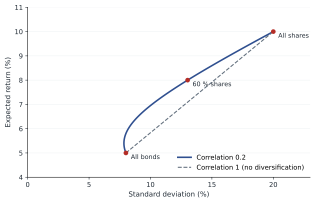
An investor rarely holds one asset. The return on a portfolio is the weighted average of the returns on its assets, but its risk is generally less than the weighted average of their risks, because the assets do not move perfectly together. How much less depends on the correlation between them, which ranges from −1 (always moving in opposite directions) to +1 (moving in lockstep). For two assets with weights \( w_1 \) and \( w_2 \), standard deviations \( \sigma_1 \) and \( \sigma_2 \) and correlation \( \rho \), the portfolio variance is given below. Unless the correlation is +1, combining the assets reduces risk below the weighted average.
Worked problem
Two-asset portfolio
A portfolio is 60 % in share fund A (expected return 10 %, standard deviation 20 %) and 40 % in bond fund B (expected return 5 %, standard deviation 8 %). Find the expected return and standard deviation if the correlation is 0.2, and compare with correlation 1.
Show solution
- Expected return = 0.6 × 10 + 0.4 × 5 = 8.0 %.
- Variance (ρ = 0.2) = 0.36 × 0.04 + 0.16 × 0.0064 + 2 × 0.6 × 0.4 × 0.2 × 0.20 × 0.08 = 0.0144 + 0.001024 + 0.001536 = 0.01696.
- Standard deviation = √0.01696 = 13.02 %.
- With ρ = 1: σ = 0.6 × 20 + 0.4 × 8 = 15.2 %.
Answer: Low correlation cuts the portfolio's risk from 15.2 % to 13.0 % with no loss of expected return. That is the free lunch of diversification.
As more assets are added, the risk that is specific to each company, such as a failed product, a lawsuit or a strike, tends to cancel out. This is unsystematic, diversifiable or firm-specific risk. What remains is the risk that affects all companies to some degree: recessions, interest rate changes, inflation, pandemics and wars. This is systematic or market risk, and no amount of diversification within the market removes it. Studies of portfolios of randomly chosen shares show that most of the benefit of diversification is achieved with a few dozen holdings, although concentrated markets and correlated industries may require more.
# Risk of equally weighted portfolios of n similar shares
# Each share: standard deviation 35 %, average correlation with others 0.25
import math
sigma, rho = 0.35, 0.25
for n in (1, 2, 5, 10, 20, 50, 100, 1000):
    var = sigma ** 2 / n + (1 - 1 / n) * rho * sigma ** 2
    print(f"{n:5d} shares: portfolio standard deviation {math.sqrt(var) * 100:5.1f} %")
print(f"limit (systematic risk only): {math.sqrt(rho) * sigma * 100:.1f} %") 1 shares: portfolio standard deviation 35.0 %
2 shares: portfolio standard deviation 27.7 %
5 shares: portfolio standard deviation 22.1 %
10 shares: portfolio standard deviation 20.0 %
20 shares: portfolio standard deviation 18.8 %
50 shares: portfolio standard deviation 18.0 %
100 shares: portfolio standard deviation 17.8 %
1000 shares: portfolio standard deviation 17.5 %
limit (systematic risk only): 17.5 %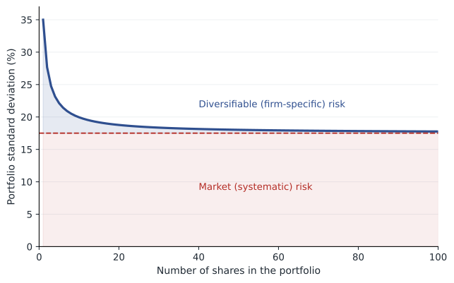
Systematic risk and beta
If investors can diversify away firm-specific risk cheaply, by holding broad index funds for example, then competition among them means they will not be paid for bearing it. The reward for risk should depend only on an asset's systematic risk: how much it contributes to the risk of a well-diversified portfolio. That contribution is measured by beta, the sensitivity of the asset's return to the return on the market portfolio. A share with a beta of 1 tends to move one-for-one with the market; a beta of 1.5 means it tends to rise 1.5 % when the market rises 1 % and fall 1.5 % when it falls 1 %; a beta of 0.5 means half the market's movement. Utilities and consumer staples typically have low betas; technology and resource companies often high ones.
In practice, beta is estimated by regressing the share's past returns on the market's returns, usually using five years of monthly data or two years of weekly data, against a broad index such as the S&P/TSX Composite or the S&P 500. Estimates are noisy, so analysts often adjust them toward 1, or use the average beta of several comparable firms. A share can have high total risk but a low beta, if most of its volatility is firm-specific, such as a small gold explorer whose fortunes depend on one drill program.
# Estimating beta from 60 months of simulated returns
import random, statistics
random.seed(2010)
true_beta = 1.3
market = [random.gauss(0.008, 0.045) for _ in range(60)]
stock = [0.002 + true_beta * m + random.gauss(0, 0.06) for m in market]
mm, ms = statistics.mean(market), statistics.mean(stock)
cov = sum((m - mm) * (s - ms) for m, s in zip(market, stock)) / 59
beta = cov / statistics.variance(market)
corr = cov / (statistics.stdev(market) * statistics.stdev(stock))
print(f"estimated beta {beta:.2f} (true value {true_beta})")
print(f"correlation with market {corr:.2f}; share of variance that is systematic {corr ** 2:.0%}")estimated beta 1.51 (true value 1.3) correlation with market 0.85; share of variance that is systematic 73%
The capital asset pricing model
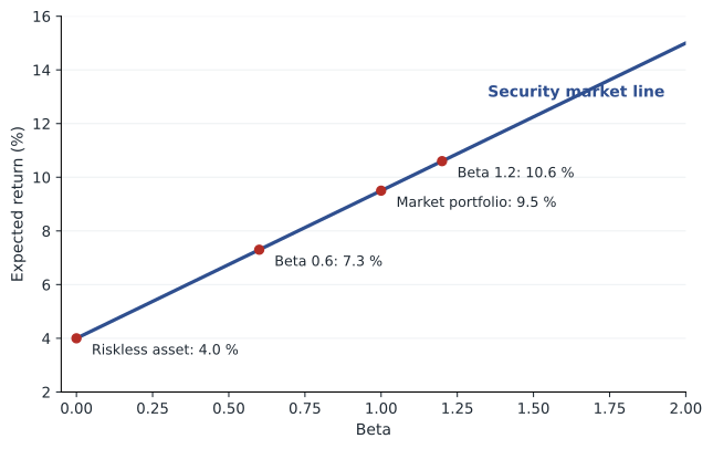
The capital asset pricing model, developed in the 1960s by William Sharpe and others, turns these ideas into a formula for expected return. If investors hold diversified portfolios and markets are competitive, every asset's expected return equals the riskless rate plus its beta times the market risk premium, the expected return on the market minus the riskless rate. Plotted against beta, this relation is the security market line.
Worked problem
Using the CAPM
The yield on 10-year Government of Canada bonds is 3.9 %, the market risk premium is estimated at 5.5 %, and a company's beta is 1.2. What return should investors expect on its shares? What about a share with a beta of 0.6?
Show solution
- Beta 1.2: E(R) = 3.9 + 1.2 × 5.5 = 10.5 %.
- Beta 0.6: E(R) = 3.9 + 0.6 × 5.5 = 7.2 %.
Answer: The higher-beta share must offer a higher expected return to compensate for its greater contribution to the risk of a diversified portfolio. The inputs are illustrative estimates for late 2026.
The CAPM is a simplification. Its assumptions, such as investors who care only about mean and variance, can borrow at the riskless rate and agree on expectations, are unrealistic, and empirical tests find that the relation between beta and average returns is flatter than the model predicts, while other characteristics, such as size, value and momentum, help explain returns. Multifactor models, such as the Fama-French models, extend the CAPM, and FIN-301 covers them. Despite its flaws, the CAPM remains the most widely used method for estimating the cost of equity in practice, because it is simple, its logic is sound, and the alternatives are not clearly more reliable for an individual company.
Implications for the firm
Three implications matter for corporate finance. First, the discount rate for a project should reflect the project's systematic risk, not the total risk of its cash flows and not the firm's overall risk if the project is different from the firm's typical business. Second, diversification by the firm, for example a conglomerate buying unrelated businesses to smooth its earnings, does not create value for shareholders who can diversify more cheaply themselves; any value from mergers must come from cash flow improvements. Third, risk that shareholders can diversify away still matters to managers, employees, lenders and suppliers, and can affect the firm through financial distress costs, as lesson 12 shows, so risk management can still create value even if diversifiable risk carries no premium in the cost of capital.
Common mistakes
MistakeThe arithmetic average return shows how fast an investment grew.
InsteadThe geometric average measures compound growth; the arithmetic average forecasts a single period.
MistakeA portfolio's risk is the weighted average of its assets' risks.
InsteadIt is lower unless the assets are perfectly correlated.
MistakeA share with high volatility must have a high expected return.
InsteadOnly systematic risk, measured by beta, is rewarded; firm-specific volatility is not.
MistakeFirms create value for shareholders by diversifying into unrelated businesses.
InsteadShareholders can diversify cheaply themselves; diversification alone adds no value.
MistakeThe CAPM gives the exact cost of equity.
InsteadIt is an estimate with uncertain inputs; treat results as approximate.
Summary and key terms
- Holding period return = (income + price change) ÷ starting price; geometric averages measure past compound growth.
- Standard deviation measures total risk; real returns have fatter tails than the normal distribution.
- Historically, shares have outperformed bonds and bills, with much higher volatility; the equity risk premium is a few percentage points a year.
- Diversification reduces risk because assets are imperfectly correlated; firm-specific risk can be diversified away, market risk cannot.
- Beta measures an asset's sensitivity to market movements and its contribution to diversified portfolio risk.
- CAPM: E(R) = Rf + β[E(Rm) − Rf]; the security market line plots it.
- Project discount rates should reflect the project's systematic risk.
- Holding period return
- Income plus price change, divided by the starting price.
- Geometric mean return
- The constant compound rate that produces the same ending wealth.
- Standard deviation
- A measure of the dispersion of returns around their mean.
- Equity risk premium
- The expected return on shares minus the riskless rate.
- Correlation
- A measure from −1 to +1 of how two returns move together.
- Diversification
- Reducing risk by combining assets that do not move together perfectly.
- Systematic risk
- Risk that affects the whole market and cannot be diversified away.
- Unsystematic risk
- Firm-specific risk that can be diversified away.
- Beta
- The sensitivity of an asset's return to the market return.
- Security market line
- The CAPM relation between beta and expected return.
Practice problems
Work each problem on paper first, then reveal the answer to check.
A share bought at $50 pays a $2 dividend and ends at $54. Return?
Show answer
12 %.
Returns of +20 % and −20 %. Arithmetic and geometric means?
Show answer
0 % and −2.02 %.
Returns 10 %, 4 %, −2 %, 12 %. Sample standard deviation?
Show answer
Mean 6 %; σ ≈ 6.32 %.
50/50 portfolio of assets with σ 30 % and 10 %, ρ = 0. Portfolio σ?
Show answer
√(0.0225 + 0.0025) = 15.8 %.
Same portfolio with ρ = −1?
Show answer
|0.15 − 0.05| = 10 %.
Covariance with market 0.0036; market variance 0.0024. Beta?
Show answer
1.5.
Rf 4 %, market risk premium 6 %, beta 0.8. CAPM expected return?
Show answer
8.8 %.
Why is firm-specific risk not rewarded?
Show answer
Investors can diversify it away at little cost.
A conglomerate buys an unrelated business to smooth earnings. Does this help shareholders?
Show answer
Not by itself; shareholders can diversify on their own.
Portfolio task: download five years of monthly returns for a share and the market index and estimate its beta.
Show answer
Answers vary; state the index, period and source.
Lesson quiz · 5 questions
Score 60% or more to complete this lesson.
Create a free account to save your progress, take quizzes and earn a certificate.