Analog values, scaling and PID control in PLCs

Process control is about holding a variable, a temperature, pressure, level or flow, at a setpoint despite disturbances. PLCs read analog measurements, compare them with setpoints, and adjust valves, heaters and drive speeds to keep the process where it should be. Doing this well requires correctly scaled and validated measurements, sensible alarms, and a properly configured and tuned PID control loop. Electricians increasingly work on these systems, whether wiring and checking analog loops, setting up drive speed references, or helping tune a temperature loop on a machine. This lesson covers scaling raw analog values to engineering units, validating and filtering signals, process alarms with deadbands, the PID algorithm as implemented in PLCs, controller action and modes, tuning methods, and common practical problems.

Scaling

Analog input modules deliver raw numbers whose range depends on the module and its configuration (for example 0 to 32,000, 6,242 to 31,208, or 4.0 to 20.0 mA). The program converts them to engineering units with a linear equation through two known points:

where x is the raw value, (x1, y1) and (x2, y2) are the raw and engineering values at the low and high ends of the range. Many PLCs provide scaling instructions (SCP, SCALE, NORM_X and SCALE_X) or allow scaling to be configured in the module. Analog outputs are scaled in reverse, from engineering units (such as 0 to 100 % valve position or 0 to 60 Hz) to raw output values.

Validating and filtering signals

A control system should never trust a measurement blindly. Validation checks include out-of-range detection (raw values below 4 mA or above 20 mA, or NAMUR fault levels, indicating broken wires or failed transmitters), rate-of-change limits (a tank level cannot really jump 30 % in one second), comparison of redundant sensors, and module diagnostic bits. When a measurement is invalid, the program should raise an alarm and move to a defined safe action, such as holding the last good value, switching to manual, or shutting down, rather than controlling on a bad signal.

Noisy signals are smoothed with filters: a first-order (exponential) filter, y_new = y_old + α(x − y_old), or a moving average over several samples. Filtering must be modest, because heavy filtering adds lag that degrades control and delays alarms. It is better to fix the source of noise (wiring, grounding, shielding) than to hide it with filters.

Process alarms

Analog alarms typically include high-high, high, low and low-low limits. To prevent alarms chattering when the value hovers near a limit, alarms use a deadband: an alarm that activates at 90 % clears only when the value falls below, say, 88 %. Delays (Lesson 8) suppress brief excursions. Alarm management principles apply: every alarm should require an operator response, alarms should be prioritized, and nuisance alarms should be eliminated, because operators flooded with meaningless alarms miss important ones. Critical safety trips (such as high-high pressure shutdowns) often belong in independent safety systems rather than the basic control PLC (Lesson 11).

The PID algorithm

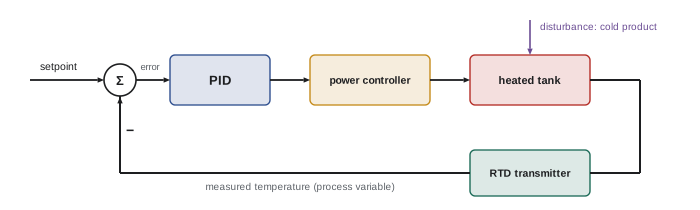
The PID controller (introduced in AI-450 for robots and familiar from many fields) calculates its output from the error between the setpoint (SP) and the process variable (PV). PLC PID instructions commonly use the "standard" or "ideal" form:

where CO is the controller output, Kc is the controller gain (sometimes expressed as proportional band, PB = 100 / Kc in percent), Ti is the integral (reset) time and Td is the derivative time. Some PLCs use the "independent" form with separate Kp, Ki and Kd gains, and units differ between manufacturers (for example integral in minutes per repeat or repeats per minute), so tuning values cannot be copied between platforms without conversion.

• Proportional action responds immediately to error but, alone, leaves a steady-state offset in most processes.
• Integral action removes offset by accumulating error over time; too much integral causes oscillation.
• Derivative action responds to the rate of change, adding anticipation; it is useful on slow processes such as temperature but amplifies noise, and is usually left at zero on flow and pressure loops. Many PLCs compute derivative on PV rather than on error, avoiding output spikes when the setpoint changes.

Action, modes and limits

Controller action must match the process. In reverse action, an increasing PV decreases the output, as for a heating loop (temperature rising means less heat) or a fill valve on a level loop. In direct action, increasing PV increases the output, as for a cooling loop or a drain valve on a level loop. Choosing the wrong action makes the loop run away to full or zero output.

PID instructions have manual and automatic modes. In manual, the operator sets the output directly; in automatic, the PID calculates it. Bumpless transfer initializes the controller so switching from manual to automatic does not jolt the output. Other important settings include output limits (for example 0 to 100 %, or a minimum speed for a pump), anti-reset windup (stopping integral accumulation when the output is limited), setpoint limits and ramping, the loop update time (which should be consistent and appropriate to the process, often 100 ms to 1 s), and cascade arrangements, where one controller's output becomes another's setpoint (for example a temperature controller setting a steam flow controller's setpoint).

Tuning

Tuning sets Kc, Ti and Td for good performance: responding promptly to setpoint changes and disturbances without excessive overshoot or oscillation, and without wearing out valves by constant movement. Common approaches:

• Open-loop step test: with the controller in manual, step the output (for example by 10 %) and record the PV response. Estimate the process gain K (change in PV divided by change in output, in consistent units), the dead time θ (delay before the PV starts to move) and the time constant τ (time to reach 63 % of the final change after the dead time).
• Lambda (internal model) tuning for self-regulating processes: choose a desired closed-loop time constant λ (often 1 to 3 times τ for a smooth, robust loop), then set Kc = τ / (K(λ + θ)) and Ti = τ, with Td = 0. It gives smooth, non-oscillatory responses and is widely used in process industries.
• Ziegler-Nichols and related methods give more aggressive tunings, which may oscillate and are usually softened in practice.
• Auto-tune functions in many PLCs and controllers perform tests automatically and suggest parameters, which should still be checked.

Common practical problems

• Valve or actuator problems such as sticking (stiction), backlash or undersized valves cause oscillation that no tuning can fix; check the final control element first.
• Measurement problems, including noise, slow sensors, wrong ranges and poor sensor location, degrade control.
• Wrong action or wrong units in the PID configuration.
• Interaction between loops, for example two loops fighting over the same process.
• Loops left in manual: surveys commonly find that a significant fraction of plant loops run in manual or perform poorly, wasting energy and quality.
• Analog outputs to drives: when a PLC sends a speed reference to a drive as 4–20 mA or 0–10 V, both the PLC scaling and the drive's analog input settings (minimum and maximum frequency for the signal range) must match, and the signal should be checked end to end.

Drives and analog control

Variable frequency drives are among the most common final control elements in process loops. A PLC can command a drive through an analog output (4–20 mA or 0–10 V), through discrete inputs for preset speeds, or over an industrial network, which also allows reading actual speed, current, faults and other data. When a drive controls a pump or fan in a PID loop, the drive's own acceleration and deceleration ramps and minimum speed settings become part of the loop dynamics and must be considered in tuning. Some drives include their own PID controllers, which can control simple pressure or flow loops without a PLC, reducing wiring and response delays.

For pumps, a minimum speed is usually needed to maintain cooling flow and to overcome static head; below it, the pump produces no flow while still consuming energy. The loop output limits should reflect this. For fans and pumps, energy savings from speed control follow the affinity laws (power roughly proportional to speed cubed), which is why converting throttled systems to drive control often pays back quickly.

Finally, document each loop's configuration: ranges, action, tuning parameters, limits and the date and method of tuning. When performance changes later, this record shows what was set and why.

Example: tuning check after start-up

After tuning a loop, test it with a small setpoint change (for example 2 % to 5 % of span) and observe the response on a trend. A well-tuned loop with lambda tuning reaches the new setpoint smoothly in about four lambda periods without overshoot; an aggressive loop overshoots and oscillates; a sluggish loop creeps slowly. Also test disturbance rejection by observing how the loop responds to normal process upsets. Record the tuning, test results and date, and revisit tuning when the process changes significantly, such as new equipment or different operating ranges.