Transport, performance and quality of service

Lesson 1 described how frames and packets are built and addressed. This lesson asks a different question: how fast does the network actually feel to the applications that use it? A link may be rated at 100 Gb/s, yet a single file transfer across it crawls along at a few hundred megabits per second, or a web page that depends on a hundred servers takes ten times longer than any one of them. The answers lie in latency, in the transport protocols that pace traffic, in what happens when many senders converge on one receiver, and in how the network decides which packets go first.

These topics matter to facility engineers as well as network engineers. The distance between buildings, the choice of switches, the placement of storage and the layout of a campus all show up as latency and throughput that customers notice.

Where the time goes: the parts of latency

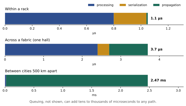
The latency of a packet is the time from when its first bit leaves the sender until its last bit reaches the receiver. It has four parts:

• Serialization delay: the time to put the bits on the wire, equal to the packet size divided by the link rate. A 1500-byte packet takes 1.2 µs at 10 Gb/s and 0.12 µs at 100 Gb/s.
• Propagation delay: the time for the signal to travel the distance. Light in optical fibre travels at about two thirds of its speed in a vacuum, roughly 204,000 km/s, so propagation adds about 4.9 µs per kilometre, usually rounded to 5 µs (Lesson 9 explains why). Copper cables are similar.
• Processing (switching) delay: the time a switch or router takes to look up and forward the packet, from a few hundred nanoseconds in a data centre switch to tens of microseconds in software.
• Queuing delay: the time a packet waits behind other packets in a switch buffer. It is zero on an idle network and can grow to milliseconds under congestion. It is the only part that changes from moment to moment, and it causes most latency problems.

Round-trip time (RTT) is the time for a packet to go out and an answer to come back, roughly twice the one-way latency. Protocols that wait for acknowledgements are governed by RTT.

TCP in brief

Most applications use TCP (Transmission Control Protocol), which turns the unreliable delivery of IP packets into a reliable, ordered byte stream. TCP numbers every byte it sends; the receiver returns acknowledgements (ACKs) saying how much it has received in order. Data that is not acknowledged within a timeout, or that the receiver signals is missing, is sent again.

TCP does not send one packet and wait. It keeps a window of unacknowledged data in flight. The window is limited by two things: the receive window the receiver advertises (how much buffer it has) and the congestion window the sender maintains (its estimate of how much the network can carry). A sender can transmit at most one window per round trip, so

The bandwidth-delay product

To fill a link, the window must be at least the bandwidth-delay product (BDP): the link rate multiplied by the RTT. The BDP is the amount of data "in the pipe" at once.

Inside a data centre the RTT is tiny, so the BDP is small: a 100 Gb/s link with a 10 µs RTT holds only 125 KB. Between cities the BDP becomes large, and every buffer, window and timer must be sized for it.

Loss and congestion control

If every sender transmitted as fast as it could, switch buffers would overflow and packets would be dropped. TCP congestion control prevents this. A new connection starts slowly and doubles its window every round trip (slow start) until it detects loss or reaches a threshold; it then grows the window steadily and cuts it sharply (typically halving it, or reducing by 30% in CUBIC, the Linux default) whenever a packet is lost. This additive-increase, multiplicative-decrease behaviour shares a bottleneck fairly between flows, but it means that loss directly limits throughput. A widely used approximation (the Mathis formula) for a long-lived flow is

where MSS is the maximum segment size (typically 1460 bytes) and \(p\) is the packet loss probability.

Newer algorithms reduce the dependence on loss. BBR, developed by Google, estimates the bottleneck bandwidth and minimum RTT and paces packets to match, rather than waiting for loss. Explicit Congestion Notification (ECN) lets switches mark packets when queues build instead of dropping them, and DCTCP (Data Center TCP, RFC 8257) uses the fraction of marked packets to slow down gently and keep queues short.

UDP and QUIC

UDP (User Datagram Protocol) adds only port numbers and a checksum to IP; it has no acknowledgements, ordering or congestion control of its own. Applications that prefer timeliness to reliability, such as voice, video calls, DNS lookups and online games, use it directly. QUIC (RFC 9000, 2021) builds a reliable, encrypted, congestion-controlled transport on top of UDP in the application itself, and carries HTTP/3. It sets up connections in fewer round trips than TCP plus TLS and avoids head-of-line blocking between streams. A large share of web traffic from the biggest content providers now uses QUIC, which matters to operators because it is encrypted end to end and cannot be inspected by middleboxes.

Buffers and incast

Every switch port has a queue. When packets arrive faster than the output link can send them, they wait in the buffer; when the buffer is full, new packets are dropped (tail drop). Data centre switch chips usually have a shared on-chip buffer of a few tens to a few hundred megabytes for the whole chip, shared among all ports, so any one port can claim only a part of it.

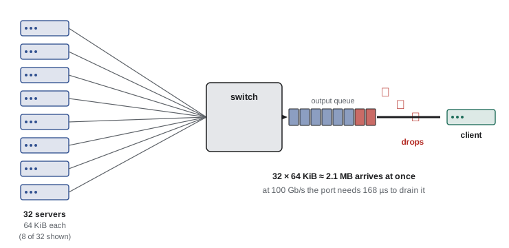
A classic data centre problem is incast: many servers answer one request at the same instant, and their responses converge on the single port leading to the requester. Distributed storage reads, search queries and AI collective operations (Lesson 11) all produce it.

Buffers are a trade-off. Deep buffers absorb bursts and help long-distance flows, but a full buffer adds delay to every packet behind it, a problem called bufferbloat: a 100 MB queue on a 10 Gb/s port adds 80 ms of latency. Data centre switches therefore use relatively shallow buffers with active queue management, while routers at the edge of the WAN, which must handle long RTTs, often use deep buffers built from external high-bandwidth memory.

Spreading traffic across paths

A leaf-spine fabric (Lesson 3) offers many equal-cost paths between any two leaves. Switches spread traffic across them with ECMP (equal-cost multipath): they hash the fields that identify a flow, usually the five-tuple of source and destination IP address, protocol and source and destination port, and use the result to pick an uplink. All packets of one flow take the same path, so they arrive in order.

Hashing works well when there are many small flows. It works poorly when a few very large flows (elephant flows) dominate, because two of them can hash onto the same link while others sit idle.

Tail latency

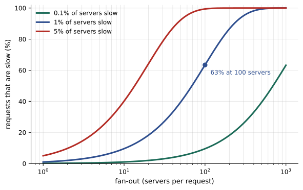
Many services answer a request by fanning it out to many servers and waiting for all of them, so the slowest server decides the response time. Average latency is then much less important than tail latency: the 99th or 99.9th percentile. Google engineers described the effect in a well-known 2013 paper, "The Tail at Scale".

Quality of service

When a link is congested, quality of service (QoS) decides whose packets wait and whose are dropped. Packets are classified by a 6-bit DSCP (Differentiated Services Code Point) field in the IP header, or by the 3-bit priority field of an Ethernet VLAN tag. Each class is placed in its own queue, and a scheduler serves the queues:

• Strict priority: one queue is always served first. It suits small amounts of latency-sensitive traffic such as voice and network control protocols, but can starve other queues if overused.
• Weighted fair queuing or deficit round robin: queues share the link in set proportions, such as 50% storage, 30% general and 20% backup.
• Policing and shaping: traffic above an agreed rate is dropped (policed) or delayed and smoothed (shaped). Carriers police customer traffic to the purchased bandwidth.
• Lossless classes: for traffic that must never be dropped, such as RDMA over Converged Ethernet (RoCE), priority flow control (PFC) pauses the sender of that class when the buffer fills (Lesson 11).

QoS cannot create capacity. It decides who suffers when there is not enough, so the first answer to persistent congestion is more bandwidth or less traffic. QoS is essential for protecting the network's own control traffic (routing protocols, management) and for converged networks that mix storage, voice and bulk data on the same links.

Measuring performance

Network performance is measured both from the network and from the hosts:

• Interface counters show utilization, errors and discards (drops) on every port. A port with rising discards is congested; a port with rising CRC errors has a physical fault.
• Latency probes send test packets between many pairs of servers continuously (a "pingmesh") to map latency and loss across the fabric.
• Throughput tests such as iperf measure what a single flow or many parallel flows can achieve.
• Utilization averages hide bursts. A link averaging 30% over five minutes may be at 100% for milliseconds at a time and dropping packets; switch telemetry that reports buffer occupancy and microbursts is needed to see it (Lesson 12).