
BUS-230 · Lesson 9 of 12 · 36 min
Inventory management
Inventory is one of the largest assets on many balance sheets and one of the most visible signs of how well an operation is managed. Too little inventory means empty shelves, idle production lines and lost customers; too much ties up cash, takes up space, becomes obsolete and hides problems. A grocery chain must decide how many bananas to order for each store each day; a hospital how many units of each blood type to hold; a car dealer how many vehicles of each trim to keep on the lot; a manufacturer how many spare parts to stock for machines that rarely fail. Inventory management answers two basic questions for each item: how much to order, and when to order it.
This lesson covers the purposes and costs of inventory, measures of inventory performance, ABC analysis and record accuracy, the economic order quantity model, reorder points and safety stock, periodic review systems and the single-period (newsvendor) model. Inventory of components whose demand depends on production plans is handled with material requirements planning in lesson 10; lean approaches to reducing inventory follow in lesson 11. How inventory is valued in financial statements is covered in the accounting courses.
Why hold inventory?
Inventory serves several purposes. Cycle inventory results from ordering or producing in batches larger than immediate needs, to spread the fixed cost of each order or set-up. Safety (buffer) stock protects against uncertainty in demand and supply lead times. Anticipation inventory is built ahead of expected peaks, such as a toy maker building stock before the holiday season or a firm stockpiling ahead of a strike or tariff increase. Pipeline (in-transit) inventory is in motion between locations; by Little's Law it equals the flow rate multiplied by transit time, so long supply routes carry large pipeline inventories. Decoupling inventory between stages lets each stage run without waiting for the others.
Inventories are also classified by stage: raw materials, work in process (WIP), finished goods, and maintenance, repair and operating (MRO) supplies such as spare parts and cleaning products. Each type needs different policies. A further distinction is between independent demand, which comes from customers and must be forecast (finished goods, spare parts), and dependent demand, which can be calculated from the production plan (the four wheels needed for each wagon a toy factory plans to build). This lesson focuses on independent demand.
The costs of inventory
Three types of cost drive inventory decisions. Holding (carrying) costs are the costs of keeping inventory: the cost of capital tied up, storage space, handling, insurance, taxes, shrinkage (theft and damage) and obsolescence. They are usually expressed as an annual percentage of the item's value; rates of 20 to 30 % a year are commonly quoted, higher for perishable or fast-obsolescing items. Ordering costs are the fixed costs of placing and receiving an order (purchasing staff time, transport, receiving and inspection) or, for items made in-house, the set-up cost of changing over equipment. Shortage (stockout) costs are the costs of running out: lost sales, lost customers, expediting, and idle production.
Holding costs rise with order size, because larger orders mean more average inventory, while ordering costs fall, because fewer orders are needed. The basic inventory problem is to balance these opposing costs while keeping shortages at an acceptable level.
Measuring inventory performance
Two related measures are widely used. Inventory turnover is the cost of goods sold divided by average inventory value; higher turnover means inventory moves through the business faster. Days of supply (or days of inventory) is average inventory divided by average daily cost of goods sold, showing how many days the inventory would last. A grocery retailer may turn its inventory 15 to 20 times a year; a jewellery store may turn it once or twice. Turnover should be compared with industry peers and tracked over time, and paired with service measures such as fill rate (the percentage of demand met immediately from stock), because inventory can always be cut by accepting more stockouts.
ABC analysis and record accuracy
Most firms stock thousands of items, and they cannot manage all of them equally closely. ABC analysis applies the Pareto principle to inventory: items are ranked by annual dollar usage (annual demand multiplied by unit cost). Typically, A items are about 15 to 20 % of items but 70 to 80 % of dollar usage; B items about 30 % of items and 15 to 25 % of usage; and C items the remaining half or more of items but only 5 to 10 % of usage. A items deserve tight control, frequent review, accurate forecasts and close supplier relationships; C items can be managed with simple rules and larger, less frequent orders.
Worked problem
ABC classification
A hardware distributor reviews six items. Annual demand and unit cost: cordless drills 2,000 at $120; extension cords 6,000 at $12; tool chests 400 at $250; screw assortments 15,000 at $2; work gloves 8,000 at $3; safety glasses 3,000 at $4. Classify them.
Show solution
- Annual dollar usage: drills $240,000; tool chests $100,000; extension cords $72,000; work gloves $24,000; screw assortments $30,000; safety glasses $12,000.
- Total = $478,000. Ranked: drills 50.2 %; tool chests 20.9 %; cords 15.1 %; screws 6.3 %; gloves 5.0 %; glasses 2.5 %.
- A items: drills and tool chests (2 of 6 items, 71 % of usage).
- B item: extension cords (15 %).
- C items: screws, gloves and glasses (3 of 6 items, 14 % of usage).
Answer: Drills and tool chests are A items that deserve close control; extension cords are a B item; screws, gloves and glasses are C items that can be managed with simpler rules.
Inventory systems are only as good as their records. If the computer says 40 units are on the shelf and there are really 12, the system will not reorder in time. Cycle counting replaces the disruptive annual physical count with frequent counts of a few items each day, with A items counted most often (perhaps monthly) and C items least (perhaps once a year). Errors are investigated to find and fix their causes, such as unrecorded scrap, picking errors or theft. Barcodes and radio-frequency identification (RFID) tags improve accuracy and reduce counting effort.
The economic order quantity
The economic order quantity (EOQ) model, first published by Ford Harris in 1913, finds the order size that minimizes the sum of annual ordering and holding costs. It assumes demand is known and constant, lead time is known and constant, the whole order arrives at once, there are no quantity discounts, and no shortages are allowed. With annual demand \(D\), ordering cost \(S\) per order and holding cost \(H\) per unit per year, annual ordering cost is \((D/Q)S\) and annual holding cost is \((Q/2)H\), since average cycle inventory is half the order quantity. Total cost is minimized where the two are equal:
Worked problem
Calculating the EOQ
A distributor sells 12,000 furnace filters a year. Each order costs $80 to place and receive, and holding a filter for a year costs $4. Find the EOQ, the number of orders a year and the annual ordering and holding cost. What would ordering 1,000 at a time cost?
Show solution
- EOQ = √(2 × 12,000 × 80 ÷ 4) = √480,000 ≈ 693 filters.
- Orders a year = 12,000 ÷ 693 ≈ 17.3, or about one every three weeks.
- Ordering cost = 17.3 × $80 ≈ $1,385; holding cost = (693 ÷ 2) × $4 ≈ $1,386; total ≈ $2,771.
- At Q = 1,000: ordering = 12 × $80 = $960; holding = 500 × $4 = $2,000; total = $2,960, only about 7 % more.
Answer: The EOQ is about 693 filters, costing about $2,771 a year. The total cost curve is flat near the optimum, so ordering in convenient lots such as 700 or even 1,000 costs little extra.
The flatness of the total cost curve near the optimum is one of the most useful practical insights of the model. Errors in estimating \(S\) or \(H\), or rounding the order quantity to a convenient pallet or case size, have only a small effect on total cost. The model's most powerful message, however, comes from its formula: the EOQ falls as ordering or set-up cost falls. Lean producers (lesson 11) attack set-up costs directly, which makes small batches economic and cuts cycle inventory. Variants of the model handle production lots that arrive gradually (the economic production quantity) and quantity discounts, where the analyst compares total cost, including purchase cost, at the EOQ and at each price break.
When to order: reorder points and safety stock
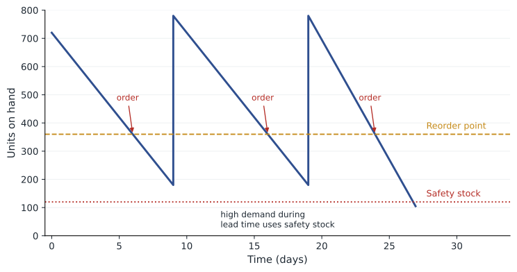
In a continuous review (or fixed-quantity) system, inventory is tracked continuously and a fixed quantity, often the EOQ, is ordered whenever the inventory position falls to the reorder point (ROP). If demand and lead time were constant, the reorder point would simply equal demand during the lead time: daily demand multiplied by lead time in days. In reality, demand varies, so the firm adds safety stock to protect against higher-than-average demand during the lead time.
If daily demand is roughly normal with mean \(\bar{d}\) and standard deviation \(\sigma_d\), and lead time \(L\) days is constant, the standard deviation of demand during the lead time is \(\sigma_d\sqrt{L}\). The safety stock for a desired cycle service level (the probability of not running out during a replenishment cycle) is \(z\) times that standard deviation, where \(z\) comes from the standard normal table: 1.28 for 90 %, 1.645 for 95 % and 2.33 for 99 %.
import math, random
from statistics import NormalDist
# EOQ and reorder point for a distributor's best-selling filter
D, S, H = 12_000, 80.0, 4.0            # units a year, $ per order, $ per unit-year
eoq = math.sqrt(2 * D * S / H)
cost = lambda q: D / q * S + q / 2 * H
print(f"EOQ = {eoq:.0f} units; annual ordering + holding cost = ${cost(eoq):,.0f}")
for q in (300, 500, 1000, 1500):
    print(f"  order {q:>5} units -> ${cost(q):,.0f}")
d_mean, d_sd, lead = 48, 10, 9           # daily demand and lead time in days
sd_lt = d_sd * math.sqrt(lead)
print(f"Demand during lead time: mean {d_mean*lead}, std dev {sd_lt:.0f}")
for level in (0.90, 0.95, 0.99):
    z = NormalDist().inv_cdf(level)
    ss = z * sd_lt
    print(f"  service {level:.0%}: z = {z:.2f}, safety stock {ss:.0f}, reorder point {d_mean*lead+ss:.0f}, holding ${ss*H:,.0f}/yr")
# Newsvendor: how many croissants to bake each morning
price, cost_u, salvage = 3.00, 0.90, 0.40
cu, co = price - cost_u, cost_u - salvage
cr = cu / (cu + co)
q_star = NormalDist(200, 40).inv_cdf(cr)
print(f"Critical ratio {cr:.3f}; optimal bake {q_star:.0f}")
random.seed(230)
days = [max(0, round(random.gauss(200, 40))) for _ in range(5000)]
def profit(q):
    return sum(price * min(q, d) + salvage * max(q - d, 0) - cost_u * q for d in days) / len(days)
for q in (180, 200, 220, 235, 260, 280):
print(f" bake {q}: average daily profit ${profit(q):.2f}")EOQ = 693 units; annual ordering + holding cost = $2,771 order 300 units -> $3,800 order 500 units -> $2,920 order 1000 units -> $2,960 order 1500 units -> $3,640 Demand during lead time: mean 432, std dev 30 service 90%: z = 1.28, safety stock 38, reorder point 470, holding $154/yr service 95%: z = 1.64, safety stock 49, reorder point 481, holding $197/yr service 99%: z = 2.33, safety stock 70, reorder point 502, holding $279/yr Critical ratio 0.808; optimal bake 235 bake 180: average daily profit $357.61 bake 200: average daily profit $378.99 bake 220: average daily profit $390.32 bake 235: average daily profit $393.01 bake 260: average daily profit $388.86 bake 280: average daily profit $381.05
The output confirms the EOQ calculation and shows the flat cost curve: ordering 500 or 1,000 at a time costs only about 5 to 7 % more than the optimum. For the reorder point, the filter sells 48 units a day on average with a standard deviation of 10, and the supplier's lead time is 9 days, so expected lead-time demand is 432 units with a standard deviation of 30. Raising the service level from 90 % to 99 % nearly doubles the safety stock, from 38 to 70 units; each extra percentage point of service costs more than the last. The final part of the output applies the newsvendor model, explained below.
Worked problem
Setting a reorder point
A hospital uses an average of 20 boxes of a sterile dressing a day, with a standard deviation of 6 boxes. The supplier's lead time is 4 days. The hospital wants a 98 % cycle service level (z = 2.05). Find the safety stock and the reorder point.
Show solution
- Expected demand during lead time = 20 × 4 = 80 boxes.
- Standard deviation during lead time = 6 × √4 = 12 boxes.
- Safety stock = 2.05 × 12 ≈ 24.6, rounded up to 25 boxes.
- Reorder point = 80 + 25 = 105 boxes.
Answer: The hospital should reorder when stock falls to 105 boxes, which includes 25 boxes of safety stock to give a 98 % chance of not running out before the delivery arrives.
When lead times also vary, safety stock must cover that uncertainty too, and for unreliable suppliers it can dominate. This is one reason firms value reliable delivery so highly (lesson 2) and why disruptions in global shipping since 2020 led many to raise safety stocks. Service level choices should reflect the cost of a stockout: high for critical medical supplies or items whose absence stops a production line, lower for items with close substitutes.
Periodic review systems
In a periodic review (or fixed-interval) system, inventory is checked at fixed intervals, such as every Monday, and an order is placed to bring the inventory position up to a target level. The order quantity varies with recent demand. Periodic review is convenient when many items are ordered from the same supplier, when deliveries follow fixed schedules or when continuous tracking is impractical, as in many small retailers and vending operations. Because inventory is not watched between reviews, the target level must cover demand over the review period plus the lead time, which requires more safety stock than a continuous system for the same service level.
| Feature | Continuous review (fixed quantity) | Periodic review (fixed interval) |
|---|---|---|
| When to order | When inventory position reaches the reorder point | At fixed review intervals |
| How much to order | Fixed quantity, often the EOQ | Variable: target level minus inventory position |
| Protection period for safety stock | Lead time | Review period plus lead time |
| Safety stock needed | Lower | Higher |
| Record-keeping | Continuous tracking needed | Counts only at review times |
| Typical use | A items, critical items, items with scanning systems | Many items from one supplier, fixed delivery routes |
The single-period (newsvendor) model
Some items can be sold only during a single period, after which they lose most of their value: newspapers, fresh baked goods, flowers for Valentine's Day, seasonal fashions, event programs. Ordering too few loses profitable sales; ordering too many leaves unsold stock that must be discarded or marked down. The newsvendor model balances these two costs. The cost of understocking, \(C_u\), is the profit lost on each unit of unmet demand (price minus cost). The cost of overstocking, \(C_o\), is the loss on each unsold unit (cost minus salvage value). The optimal order quantity is the one at which the probability of demand being less than or equal to the quantity equals the critical ratio:
Worked problem
How many croissants to bake
A café sells croissants for $3.00 that cost $0.90 to make. Unsold croissants are sold to a discount outlet the next day for $0.40. Daily demand is approximately normal with a mean of 200 and a standard deviation of 40. How many should the café bake each morning?
Show solution
- Cu = 3.00 − 0.90 = $2.10; Co = 0.90 − 0.40 = $0.50.
- Critical ratio = 2.10 ÷ (2.10 + 0.50) ≈ 0.808.
- The z-value with 80.8 % of the normal distribution below it is about 0.87.
- Q* = 200 + 0.87 × 40 ≈ 235 croissants.
Answer: The café should bake about 235 croissants, more than average demand, because a lost sale costs four times as much as a leftover. The simulation in the code confirms that average profit peaks near 235.
The newsvendor logic applies well beyond bakeries: airlines overbooking seats, hospitals deciding how many beds to staff, fashion retailers placing a single pre-season order, and firms setting capacity for a product launch. Whenever the cost of having too little differs from the cost of having too much, the best decision is not to plan for average demand.
Managing inventory across the business
Several practices reduce the inventory needed for a given service level. Pooling inventory in fewer locations reduces total safety stock, because random variations in different markets partly cancel. Shortening and stabilizing lead times reduces both safety and pipeline stock. Better forecasts (lesson 6) reduce the uncertainty safety stock must cover. Postponement (lesson 3) holds generic stock and customizes late. Vendor-managed inventory (VMI) lets the supplier monitor the customer's stock and decide when to replenish, which can reduce stockouts and inventory for both. Consignment stock, owned by the supplier until used, shifts holding cost but not the underlying inventory.
Common mistakes
MistakeTreating every item the same way.
InsteadUse ABC analysis to focus control effort on the high-value A items.
MistakeInsisting on the exact EOQ value.
InsteadRound to convenient lot sizes; the total cost curve is flat near the optimum.
MistakeSetting the reorder point equal to average lead-time demand.
InsteadAdd safety stock to cover variation, or the item will run out about half the time.
MistakePlanning for average demand on perishable items.
InsteadUse the critical ratio, which may call for more or less than average demand.
MistakeJudging inventory performance by turnover alone.
InsteadPair turnover with fill rate or service level.
MistakeIgnoring record accuracy.
InsteadUse cycle counting and fix the causes of discrepancies.
Summary and key terms
- Inventory serves as cycle, safety, anticipation, pipeline and decoupling stock.
- Holding, ordering and shortage costs drive inventory decisions.
- Turnover and days of supply measure how fast inventory moves; fill rate measures service.
- ABC analysis ranks items by annual dollar usage to focus management attention.
- Cycle counting keeps inventory records accurate.
- The EOQ, √(2DS ÷ H), minimizes ordering plus holding cost; the cost curve is flat near the optimum.
- The reorder point equals expected lead-time demand plus safety stock, z σd √L.
- Periodic review systems need more safety stock than continuous review systems.
- The newsvendor model sets single-period orders where P(demand ≤ Q) equals Cu ÷ (Cu + Co).
- Cycle inventory
- Inventory that results from ordering in batches larger than immediate needs.
- Safety stock
- Extra inventory held to protect against uncertainty in demand or supply.
- Holding cost
- The cost of keeping one unit in inventory for a period.
- Inventory turnover
- Cost of goods sold divided by average inventory.
- ABC analysis
- Classifying inventory items by annual dollar usage.
- Cycle counting
- Counting a small number of items frequently to keep records accurate.
- Economic order quantity
- The order size that minimizes total annual ordering and holding costs.
- Reorder point
- The inventory level at which a new order is placed.
- Cycle service level
- The probability of not running out of stock during a replenishment cycle.
- Critical ratio
- Cu ÷ (Cu + Co), the target probability in the newsvendor model.
Practice problems
Work each problem on paper first, then reveal the answer to check.
Name three purposes of holding inventory.
Show answer
Cycle stock, safety stock and anticipation stock (also pipeline and decoupling).
Cost of goods sold is $6 million and average inventory $1 million. Find turnover and days of supply.
Show answer
Turnover 6; days of supply ≈ 61.
D = 5,000, S = $50, H = $2. Find the EOQ.
Show answer
√250,000 = 500 units.
For the same item, what is total annual ordering and holding cost at the EOQ?
Show answer
10 orders × $50 + 250 × $2 = $1,000.
Daily demand averages 30 with standard deviation 5; lead time is 16 days; z = 1.645. Find the ROP.
Show answer
480 + 1.645 × 20 ≈ 513.
Why does a periodic review system need more safety stock?
Show answer
It must protect against variation over the review period plus the lead time.
A Christmas tree costs $25, sells for $60 and has no salvage value. What is the critical ratio?
Show answer
35 ÷ 60 ≈ 0.58.
If ordering costs fall sharply, what happens to the EOQ?
Show answer
It falls, making smaller, more frequent orders economic.
Why does pooling inventory reduce safety stock?
Show answer
Random demand variations in different markets partly cancel.
Portfolio task: classify ten items in a store or your home pantry by annual dollar usage and propose a review policy for each class.
Show answer
Answers vary; show usage, ABC classes and policies.
Lesson quiz · 5 questions
Score 60% or more to complete this lesson.
Create a free account to save your progress, take quizzes and earn a certificate.