
BUS-230 · Lesson 6 of 12 · 30 min
Forecasting demand
Almost every operations decision rests on a forecast. A bakery decides how much dough to mix tonight based on how many loaves it expects to sell tomorrow; a hospital schedules nurses for next month based on expected admissions; a carmaker sizes a new plant based on demand ten years out. Forecasts are always wrong to some degree, because the future is uncertain, but some forecasts are much less wrong than others, and the size and direction of the errors can be measured, tracked and planned for. The goal of forecasting is not perfect prediction but forecasts that are good enough, unbiased and accompanied by a sense of their likely error.
This lesson covers the purposes and horizons of forecasts, qualitative methods, time-series methods (moving averages, exponential smoothing, trend projection and seasonal indices), causal methods, the measurement of forecast accuracy and bias, and forecasting practice in organizations. The statistical foundations, including regression, are developed in BUS-110 and STAT-141; this lesson focuses on applying them to operations.
Purposes and horizons
Forecasts serve different decisions over different time horizons. Short-range forecasts, up to about three months, support scheduling, staffing, purchasing and inventory replenishment; they are usually made for individual products or locations and updated frequently. Medium-range forecasts, from three months to about two years, support aggregate planning, budgeting and workforce decisions (lesson 10); they are usually made for product families. Long-range forecasts, beyond two years, support capacity, location and new product decisions (lessons 4 and 5); they are made for whole markets and rely more on judgement and scenarios.
Several principles hold across horizons. Forecasts are more accurate for groups of items than for individual items, because random variations partly cancel: total weekly demand for milk at a supermarket is easier to predict than demand for one brand of organic 2 % milk. Forecasts are more accurate for shorter horizons. And a forecast should be paired with an estimate of its error, because a plan that works only if the forecast is exactly right is a fragile plan.
Qualitative methods
Qualitative or judgement-based methods rely on human judgement and are used when historical data are scarce or irrelevant, as with a new product, a new market or a sudden change in conditions. A jury of executive opinion pools the views of senior managers, sometimes combined with statistical models; it is fast but vulnerable to the views of the most powerful person in the room. A sales force composite adds up the estimates of individual salespeople for their territories; salespeople know customers well but may lowball forecasts that become quotas. A consumer market survey asks potential customers about their purchase intentions, which tend to be optimistic (BUS-220). The Delphi method collects anonymous forecasts from a panel of experts over several rounds, sharing a summary after each round, so that the group converges without being dominated by any individual.
Judgement also plays a role alongside quantitative methods. Planners routinely adjust statistical forecasts for known future events, such as a promotion, a competitor's store opening or a change in regulations. Research shows these adjustments help when they are based on specific information and hurt when they reflect optimism or general hunches. Good practice is to record each adjustment and its reason and to check later whether it improved accuracy.
Time-series components
Time-series methods forecast the future from the past pattern of the variable itself. A demand series usually combines several components. Trend is the long-run upward or downward movement. Seasonality is a pattern that repeats over a fixed period, such as a day of the week, a month or a quarter: snow tires sell in autumn, restaurant traffic peaks at lunch and dinner. Cycles are longer, irregular swings related to the business cycle. Random variation is the unpredictable remainder. The art of time-series forecasting is to model the systematic components and leave only random variation.
Naive forecasts and moving averages
The simplest method, the naive forecast, uses the last period's actual demand as the next period's forecast. It is surprisingly hard to beat for some series and is a useful benchmark: a sophisticated method that cannot beat the naive forecast is not adding value. A simple moving average uses the average of the most recent \(n\) periods. Longer averages smooth out more random variation but react more slowly to real changes. A weighted moving average gives more weight to recent periods, for example 0.5, 0.3 and 0.2 for the last three periods. All moving averages lag behind a trend, because they average past values that were lower (in a rising trend) than current values.
Exponential smoothing
Exponential smoothing is the most widely used short-term forecasting method in practice because it is simple, needs little data storage and adapts to change. The new forecast is the old forecast plus a fraction \(\alpha\) (the smoothing constant, between 0 and 1) of the last forecast error:
A high \(\alpha\), such as 0.5, responds quickly to changes but also chases random noise; a low \(\alpha\), such as 0.1, produces a smooth forecast that responds slowly. Values between 0.1 and 0.3 are common for stable series. Like moving averages, simple exponential smoothing lags behind a trend. Extensions add a trend term (Holt's method) and seasonal factors (Holt–Winters), and these models underlie many commercial forecasting systems.
Worked problem
Exponential smoothing by hand
A bakery sold 120, 132, 126, 140, 136 and 150 loaves of sourdough in six successive weeks. Using α = 0.3 and an initial forecast of 120 for week 1, forecast weeks 2 through 7. Compare with a 3-week moving average forecast for week 7.
Show solution
- F2 = 120 + 0.3 × (120 − 120) = 120.0.
- F3 = 120 + 0.3 × (132 − 120) = 123.6; F4 = 123.6 + 0.3 × (126 − 123.6) = 124.3.
- F5 = 124.3 + 0.3 × (140 − 124.3) ≈ 129.0; F6 = 129.0 + 0.3 × (136 − 129.0) ≈ 131.1.
- F7 = 131.1 + 0.3 × (150 − 131.1) ≈ 136.8.
- 3-week moving average for week 7 = (140 + 136 + 150) ÷ 3 = 142.0.
Answer: Exponential smoothing forecasts about 137 loaves for week 7 and the moving average 142. Both lag the rising trend; a method with a trend term would forecast higher.
Trend projection and seasonality
When a series has a clear trend, a trend line fitted by least squares regression (the method covered in BUS-110 and STAT-141) can be projected forward: \(\hat{y} = a + b\,t\), where \(t\) is the time period, \(b\) the slope (the average change per period) and \(a\) the intercept. Trend projection works well for medium-range forecasts of steadily growing or declining series but can badly overshoot when growth slows, so long-range trend projections should be treated with caution.
Seasonal patterns are captured with seasonal indices. A seasonal index is the average demand in a season divided by the average demand across all seasons; an index of 1.30 for December means December demand is typically 30 % above an average month. To forecast, the analyst forecasts the average (deseasonalized) level, often with a trend line, and multiplies by the seasonal index. Retailers, utilities, tourism operators and food manufacturers all depend on seasonal indices, often at weekly or daily granularity.
Worked problem
Seasonal indices for a ski shop
A ski and bike shop recorded quarterly sales (in thousands of dollars) over two years: year 1: Q1 80, Q2 30, Q3 50, Q4 240; year 2: Q1 100, Q2 40, Q3 60, Q4 280. Calculate seasonal indices and forecast each quarter of year 3 if total annual sales are expected to reach $480,000.
Show solution
- Average for each quarter: Q1 (80 + 100) ÷ 2 = 90; Q2 35; Q3 55; Q4 260.
- Average quarter overall = (90 + 35 + 55 + 260) ÷ 4 = 110.
- Indices: Q1 90 ÷ 110 ≈ 0.82; Q2 0.32; Q3 0.50; Q4 2.36 (they sum to 4).
- Year 3 average per quarter = 480 ÷ 4 = 120.
- Forecasts: Q1 120 × 0.82 ≈ 98; Q2 ≈ 38; Q3 60; Q4 ≈ 284 (thousand dollars).
Answer: Year 3 forecasts are about $98,000, $38,000, $60,000 and $284,000 for the four quarters, reflecting the strong winter peak.
Causal methods
Causal (associative) methods forecast demand from other variables believed to drive it. A home builder might forecast housing starts from interest rates and population growth; a utility might forecast electricity demand from temperature; a retailer might forecast store sales from price, promotion and local income. Linear regression with one or more explanatory variables is the standard tool. Causal models can be powerful, but they require forecasts of the explanatory variables themselves and assume that relationships observed in the past continue. Correlation alone does not prove causation, and a model with many variables can fit past data well yet forecast poorly.
Machine learning methods, such as gradient-boosted trees and neural networks, are now widely used by large retailers and platforms to forecast demand for millions of items using many inputs: price, promotions, weather, holidays, web traffic and local events. They can improve accuracy, especially for large data sets, but are harder to interpret and still need careful validation against simple benchmarks. Demand sensing uses very recent signals, such as point-of-sale data and online searches, to adjust short-term forecasts.
Measuring forecast accuracy
Forecast error is actual demand minus the forecast, \(e_t = A_t - F_t\). Several summary measures are used. The mean absolute deviation (MAD) is the average of the absolute errors and is easy to interpret in units. The mean squared error (MSE) penalizes large errors more heavily. The mean absolute percentage error (MAPE) expresses errors as a percentage of actual demand, allowing comparison across items of different sizes, but it is distorted when actual demand is close to zero. Bias, the average of the signed errors, shows whether forecasts are consistently too high or too low.
The tracking signal (TS) is the running sum of forecast errors divided by the MAD. If the forecast is unbiased, positive and negative errors cancel and the tracking signal stays near zero. A tracking signal beyond about ±4 MADs is a common warning that the forecast is biased and the method or its parameters should be reviewed. Many forecasting systems compute tracking signals for every item and flag those outside the limits for a planner's attention.
import random, statistics as st
random.seed(230)
# 24 months of demand with trend and noise (units)
demand = [round(500 + 6 * t + random.gauss(0, 25)) for t in range(24)]

def moving_average(d, n):
    return [None] * n + [sum(d[i - n:i]) / n for i in range(n, len(d))]

def exp_smooth(d, alpha):
    f = [d[0]]
    for x in d[:-1]:
        f.append(f[-1] + alpha * (x - f[-1]))
    return f

def trend_line(d):
    t = list(range(1, len(d) + 1))
    tbar, dbar = st.mean(t), st.mean(d)
    b = sum((ti - tbar) * (di - dbar) for ti, di in zip(t, d)) / sum((ti - tbar) ** 2 for ti in t)
    return dbar - b * tbar, b

def errors(actual, fc, start):
    e = [a - f for a, f in zip(actual[start:], fc[start:])]
    mad = sum(abs(x) for x in e) / len(e)
    mape = sum(abs(x) / a for x, a in zip(e, actual[start:])) / len(e)
    bias = sum(e) / len(e)
    return mad, mape, bias, sum(e) / mad

start = 12   # evaluate all methods on months 13-24
a, b = trend_line(demand[:start])
methods = {
    "3-month moving avg": moving_average(demand, 3),
    "exp smoothing a=0.2": exp_smooth(demand, 0.2),
    "exp smoothing a=0.5": exp_smooth(demand, 0.5),
    "trend (fit months 1-12)": [a + b * (t + 1) for t in range(24)],
}
print(f"Trend line from months 1-12: demand = {a:.1f} + {b:.2f} t")
print(f"{'method':<24} {'MAD':>6} {'MAPE':>6} {'bias':>6} {'TS':>6}")
for name, fc in methods.items():
    mad, mape, bias, ts = errors(demand, fc, start)
    print(f"{name:<24} {mad:6.1f} {mape:6.1%} {bias:6.1f} {ts:6.1f}")
print("Month 25 forecast from the trend line:", round(a + b * 25))Trend line from months 1-12: demand = 489.7 + 5.99 t method MAD MAPE bias TS 3-month moving avg 27.4 4.7% 12.0 5.2 exp smoothing a=0.2 35.6 5.9% 28.6 9.6 exp smoothing a=0.5 26.8 4.5% 12.4 5.5 trend (fit months 1-12) 17.6 3.1% -1.5 -1.0 Month 25 forecast from the trend line: 639
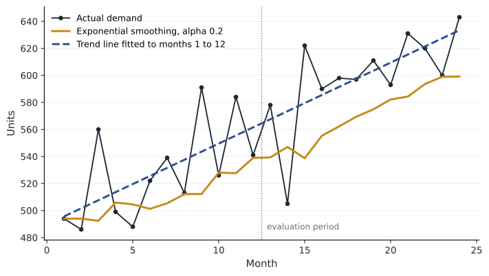
The comparison uses the first 12 months to fit or start each method and evaluates errors on the last 12 months, a simple form of out-of-sample testing. Because this series has a steady upward trend, the moving average and both smoothing forecasts run consistently low: their bias is positive and their tracking signals exceed +4, flagging the problem. The slow smoothing constant (α = 0.2) lags most. The trend line, which models the systematic growth, has the lowest MAD and MAPE and almost no bias. On a series without trend, the ranking could easily reverse, which is why methods should be compared on each item's own data.
Forecasting in practice
In organizations, forecasting is a process as well as a calculation. Many firms run a monthly demand review as part of sales and operations planning (lesson 10), where a statistical baseline is reviewed by sales, marketing and operations, adjusted for known events, and agreed as a single consensus forecast that drives all plans. Collaborative planning, forecasting and replenishment (CPFR) extends this across companies: a retailer and its supplier share point-of-sale data, promotions plans and forecasts to reduce errors and inventory on both sides.
Common problems include using sales rather than demand as the history (if the item was out of stock, sales understate demand), confusing forecasts with targets or budgets, adjusting forecasts to protect bonuses, and failing to measure accuracy at all. Forecast value added analysis compares the accuracy of each step in the process, such as the statistical forecast and the planner's adjustment, against the naive forecast, so that steps that make the forecast worse can be dropped.
| Method | Data needed | Horizon | Strengths | Weaknesses |
|---|---|---|---|---|
| Delphi and expert judgement | Expert knowledge | Medium to long | Works without history | Slow; subject to bias |
| Naive | Last period | Very short | Simple benchmark | Ignores trend and seasonality |
| Moving average | Last n periods | Short | Smooths noise | Lags trends |
| Exponential smoothing | Previous forecast and actual | Short | Adaptive, little data needed | Basic version lags trends |
| Trend and seasonal models | Several seasons of history | Short to medium | Captures systematic patterns | Can overshoot when trends change |
| Causal regression and machine learning | History of demand and drivers | Short to medium | Explains and uses drivers | Needs forecasts of drivers; risk of overfitting |
Common mistakes
MistakeUsing a forecast as a single certain number.
InsteadPair every forecast with an estimate of error and plan buffers accordingly.
MistakeForecasting from past sales when items were often out of stock.
InsteadUse demand history, adjusting for lost sales during stockouts.
MistakeApplying simple exponential smoothing to a strongly trending series.
InsteadUse a method with a trend term, such as Holt's method or a trend line.
MistakeChoosing a method by how well it fits past data.
InsteadCompare methods on data held out from fitting, and against the naive benchmark.
MistakeIgnoring a tracking signal that drifts beyond ±4.
InsteadInvestigate the bias and revise the method, its parameters or the inputs.
MistakeConfusing forecasts with sales targets.
InsteadKeep the unbiased forecast separate from targets and budgets.
Summary and key terms
- Forecasts drive scheduling, staffing, inventory, capacity and location decisions.
- Forecasts are more accurate for groups of items and shorter horizons, and should state their likely error.
- Qualitative methods include executive opinion, sales force composites, surveys and the Delphi method.
- Time series combine trend, seasonality, cycles and random variation.
- Moving averages and exponential smoothing smooth noise but lag trends; α controls responsiveness.
- Trend lines and seasonal indices capture systematic patterns; causal and machine-learning models use drivers.
- MAD, MSE and MAPE measure accuracy; bias and the tracking signal detect systematic error.
- Methods should be compared out of sample and against the naive forecast.
- Forecasting is an organizational process: consensus forecasts, CPFR and forecast value added analysis.
- Time series
- A sequence of observations of a variable taken at regular intervals.
- Seasonality
- A pattern of demand that repeats over a fixed period.
- Delphi method
- A forecasting method using anonymous expert opinions over several rounds.
- Moving average
- A forecast equal to the average of the most recent n periods.
- Exponential smoothing
- A forecast that updates the previous forecast by a fraction of the last error.
- Smoothing constant
- The weight α given to the most recent error in exponential smoothing.
- Seasonal index
- Average demand in a season divided by average demand across all seasons.
- Mean absolute deviation
- The average of the absolute forecast errors.
- Tracking signal
- The running sum of forecast errors divided by the MAD, used to detect bias.
- CPFR
- Collaborative planning, forecasting and replenishment between trading partners.
Practice problems
Work each problem on paper first, then reveal the answer to check.
Name the four components of a time series.
Show answer
Trend, seasonality, cycles and random variation.
Demand for the last three months was 200, 220 and 240. What is the 3-month moving average forecast?
Show answer
220.
The forecast was 100 and actual demand 120. With α = 0.2, what is the next forecast?
Show answer
104.
Why do moving averages lag behind a rising trend?
Show answer
They average past values, which were lower than current values.
Errors over four periods are +10, −5, +15 and +20. Find the MAD and the tracking signal.
Show answer
MAD = 12.5; TS = 40 ÷ 12.5 = 3.2.
A seasonal index is 1.25 and the deseasonalized forecast 400. What is the seasonal forecast?
Show answer
500.
Why is MAPE misleading for an item with very low demand?
Show answer
Small absolute errors become huge percentages when actual demand is near zero.
When is the Delphi method useful?
Show answer
For long-range or new-product forecasts with little data, where expert judgement is needed.
What does a tracking signal of +6 suggest?
Show answer
The forecast is consistently too low (biased) and needs review.
Portfolio task: collect 12 periods of data for a series you can observe and compare two forecasting methods using MAD.
Show answer
Answers vary; show forecasts, errors, MAD and a recommendation.
Lesson quiz · 5 questions
Score 60% or more to complete this lesson.
Create a free account to save your progress, take quizzes and earn a certificate.