
BUS-230 · Lesson 4 of 12 · 33 min
Capacity planning and queuing
Capacity is the maximum output an operation can achieve in a given period. Too little capacity loses sales, frustrates customers with long waits and burns out staff; too much capacity ties up money in idle buildings, equipment and people. Capacity decisions are among the most consequential operations decisions because they often involve large, long-lived investments: a new plant, a hospital wing, a fleet of aircraft or a data centre may take years to build and decades to pay off. In services, where output cannot be stored, capacity decisions also show up immediately in queues of waiting customers.
This lesson defines the main measures of capacity, explains strategies for timing capacity changes, shows how to evaluate expansion options with decision trees, and introduces queuing theory, which explains why waiting lines form and how to size service capacity. It builds on the bottleneck and Little's Law ideas from lesson 3.
Measuring capacity
Capacity can be measured in output units (cars per shift, patients per day) or, when outputs vary greatly, in input units (machine hours, seats, beds, staff hours). Three measures are commonly distinguished. Design capacity is the maximum output under ideal conditions. Effective capacity is the maximum output that can realistically be sustained, given the product mix, scheduling, maintenance, quality allowances and normal breaks. Actual output is what is achieved, which is usually lower still because of breakdowns, absenteeism, material shortages and quality problems.
Two ratios compare these measures. Utilization is actual output divided by design capacity; efficiency is actual output divided by effective capacity. A process can have low utilization but high efficiency if its effective capacity is well below design, for example because of frequent product changeovers. Improving efficiency means managing day-to-day problems better; improving effective capacity means reducing the structural losses, for example by shortening changeovers or improving maintenance.
Worked problem
Utilization and efficiency at a bakery
A commercial bakery's ovens can produce 12,000 loaves a day under ideal conditions. Allowing for changeovers between bread types, cleaning and planned maintenance, its effective capacity is 10,000 loaves a day. Last week it averaged 8,500 loaves a day. Calculate utilization and efficiency and interpret them.
Show solution
- Utilization = 8,500 ÷ 12,000 ≈ 70.8 %.
- Efficiency = 8,500 ÷ 10,000 = 85 %.
- About 2,000 loaves a day are lost to structural factors (changeovers, cleaning, maintenance) and 1,500 to operating problems.
- Shortening changeovers would raise effective capacity; reducing breakdowns and shortages would raise efficiency.
Answer: Utilization is about 71 % and efficiency 85 %. The bakery can gain output both by reducing structural losses and by running more reliably.
Timing capacity changes
Demand changes over time, and capacity usually comes in lumps: a plant, a production line or a shift. Three broad strategies exist for timing additions. A lead strategy adds capacity ahead of demand, so there is always a cushion; it protects sales and service in growing markets but risks idle capacity if growth stalls. A lag strategy adds capacity only after demand has clearly exceeded it; it uses capital efficiently but loses sales and may push customers to competitors. A match (or straddle) strategy adds capacity in smaller increments that alternately lead and lag demand.
The capacity cushion is the amount by which capacity exceeds expected demand, often expressed as a percentage. Firms facing uncertain or highly variable demand, or competing on speed and service, hold larger cushions: hospitals and electricity utilities need reserve capacity for peaks and emergencies. Firms in stable, cost-driven markets with expensive equipment, such as paper mills, run with small cushions. Economies of scale (lower unit costs at higher volume, from spreading fixed costs and specialization) favour large facilities, but diseconomies of scale (complexity, communication problems and transport costs) eventually set in. Many firms prefer several medium-sized facilities to one giant one.
| Strategy | How it works | Advantages | Risks |
|---|---|---|---|
| Lead | Add capacity before demand arrives | Never short of capacity; supports growth and service | Idle capacity and cost if demand falls short |
| Lag | Add capacity after demand exceeds it | High utilization; capital spent only when needed | Lost sales, long waits, overtime and burnout |
| Match (straddle) | Add smaller increments around the demand curve | Balances the two risks | Frequent changes; still periods of shortage or surplus |
Capacity in services
Services cannot build inventory to absorb demand fluctuations, so they manage both capacity and demand. On the capacity side, they use part-time and seasonal staff, cross-train employees to move between tasks, schedule shifts to follow demand patterns, share capacity with other organizations, and shift work to customers through self-service. On the demand side, they use reservations and appointments, differential pricing (cheaper matinees, off-peak fares, surge pricing), promotions in slow periods, and complementary services that keep customers busy while they wait.
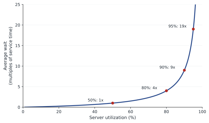
Services also face an interesting relationship between utilization and quality. A restaurant at 100 % of its seats feels rushed and service suffers; one at 20 % feels empty and unappealing. For many services, the best experience occurs at around 70 to 80 % of capacity, which leaves room to respond to customers without long waits. The queuing models later in this lesson show why waiting time rises steeply as utilization approaches 100 %.
Evaluating capacity options with decision trees
Capacity decisions are made under uncertainty about future demand. A decision tree lays out the choices (square nodes), the uncertain events with their probabilities (round nodes) and the payoffs at the end of each branch. The expected monetary value of each choice is the probability-weighted average of its payoffs, and the decision with the highest expected value is preferred if the decision maker is risk-neutral. Trees can include later decisions, such as the option to expand a small facility if demand turns out high, which often adds considerable value.
Worked problem
Choosing a warehouse expansion
A distributor can build a large expansion, a small expansion or do nothing. Demand will be high with probability 0.6 or low with probability 0.4. Net present values: large expansion $900,000 if high, −$150,000 if low; small expansion $500,000 if high, $100,000 if low; do nothing $0. Which option maximizes expected value? How does the answer change if the small expansion can later be enlarged, raising its high-demand value to $700,000?
Show solution
- EMV(large) = 0.6 × 900,000 + 0.4 × (−150,000) = 540,000 − 60,000 = $480,000.
- EMV(small) = 0.6 × 500,000 + 0.4 × 100,000 = 300,000 + 40,000 = $340,000.
- EMV(do nothing) = $0, so the large expansion is preferred.
- With the option to enlarge: EMV(small) = 0.6 × 700,000 + 0.4 × 100,000 = $460,000, now close to the large option.
- A risk-averse firm might prefer the small expansion: its worst outcome is +$100,000 rather than −$150,000.
Answer: The large expansion has the highest expected value ($480,000), but the flexible small expansion ($460,000 with the option to enlarge) comes close with far less downside risk.
Why queues form
Waiting lines, or queues, form whenever demand temporarily exceeds capacity. The surprising insight of queuing theory is that queues form even when average capacity exceeds average demand, because arrivals and service times vary. If a bank teller can serve 30 customers an hour and 24 arrive per hour on average, the teller is idle 20 % of the time, yet customers still wait, because sometimes several arrive close together or one customer takes a long time. The more variable the arrivals and service times, and the closer utilization is to 100 %, the longer the queues.
A queuing system is described by its arrival process (often modelled as random Poisson arrivals at average rate \(\lambda\)), its service process (often modelled as exponentially distributed service times at average rate \(\mu\) per server), the number of servers, the queue discipline (usually first come, first served, but sometimes priority, as in hospital triage) and the queue configuration (one line feeding several servers is generally fairer and more efficient than separate lines for each server).
The single-server model
The simplest model, called M/M/1, has Poisson arrivals, exponential service times and one server. With utilization \(\rho = \lambda / \mu\) (which must be below 1 for the queue to be stable), the key results are:
Here \(L_q\) is the average number waiting, \(W_q\) the average time waiting, \(W\) the average time in the system including service and \(L\) the average number in the system. The last relationship is Little's Law again. The formula for \(L_q\) explains the steep curve in the figure: at 50 % utilization, \(L_q = 0.5\); at 80 %, 3.2; at 90 %, 8.1; at 95 %, 18.05. Each step toward full utilization costs disproportionately more waiting.
Worked problem
A coffee drive-through
A drive-through window serves an average of 30 cars an hour (2 minutes per car, exponentially distributed), and cars arrive at random at an average of 24 an hour. Find utilization, the average number of cars waiting, the average wait and the average total time. What happens if arrivals rise to 27 an hour?
Show solution
- ρ = 24 ÷ 30 = 0.8.
- Lq = 0.8² ÷ (1 − 0.8) = 0.64 ÷ 0.2 = 3.2 cars waiting on average.
- Wq = 3.2 ÷ 24 ≈ 0.133 hours = 8 minutes; W = 8 + 2 = 10 minutes.
- At 27 cars an hour: ρ = 0.9; Lq = 0.81 ÷ 0.1 = 8.1 cars; Wq = 8.1 ÷ 27 = 0.3 hours = 18 minutes.
- A 12.5 % rise in demand more than doubles the wait, because the system was already heavily loaded.
Answer: At 24 cars an hour, customers wait 8 minutes on average; at 27 cars an hour, the wait jumps to 18 minutes. Adding a second window or speeding service would be needed to protect the experience.
Multiple servers and staffing
With several servers fed by one line (the M/M/c model), the probability that an arriving customer must wait is given by the Erlang C formula, named after the Danish engineer A. K. Erlang, who developed queuing theory for telephone exchanges around 1910. Call centres, hospital admitting desks, airport security and help desks use Erlang C to decide how many staff are needed in each period to meet a service level target, such as answering 80 % of calls within 20 seconds. The calculation is tedious by hand but simple in code or a spreadsheet.
import math

def erlang_c(lam, mu, c):
    """Probability an arrival must wait in an M/M/c queue."""
    a = lam / mu                 # offered load in erlangs
    rho = a / c
    if rho >= 1:
        return 1.0
    top = a**c / math.factorial(c) / (1 - rho)
    bottom = sum(a**k / math.factorial(k) for k in range(c)) + top
    return top / bottom

lam = 100 / 60      # 100 calls an hour, per minute
mu = 1 / 5          # 5-minute average handling time
target_sec = 20
print(" agents  util   P(wait)  avg wait (s)  answered in 20 s")
for c in range(9, 14):
    pw = erlang_c(lam, mu, c)
    wq = pw / (c * mu - lam)                      # minutes
    sl = 1 - pw * math.exp(-(c * mu - lam) * target_sec / 60)
print(f"{c:>6} {lam/(c*mu):5.0%} {pw:7.1%} {wq*60:12.0f} {sl:15.1%}") agents util P(wait) avg wait (s) answered in 20 s
9 93% 76.0% 342 27.3%
10 83% 48.8% 88 56.4%
11 76% 30.0% 34 74.9%
12 69% 17.6% 14 86.2%
13 64% 9.9% 6 92.8%With 100 calls an hour and a 5-minute handling time, the offered load is about 8.3 agents' worth of work. Nine agents keep the system stable but leave most callers waiting; each additional agent cuts waiting sharply. Eleven agents answer about 75 % of calls within 20 seconds; twelve is the smallest number that meets the 80/20 target. The manager can read off the smallest number of agents that meets the 80/20 target and then add an allowance for breaks, training and absence, often called shrinkage.
Balancing service cost and waiting cost
Choosing service capacity is an economic trade-off. More servers raise the cost of service; fewer servers raise the cost of waiting. For internal customers, waiting cost is measurable: mechanics waiting at a tool crib are paid while idle. For external customers it is harder to measure but real: lost sales, abandoned calls and damage to reputation. The total cost is minimized at the capacity where the marginal cost of another server equals the marginal reduction in waiting cost.
Perceived waits matter as much as actual waits. David Maister's principles of the psychology of waiting note that unoccupied time feels longer than occupied time, uncertain and unexplained waits feel longer than known, explained ones, unfair waits feel longer than equitable ones, and anxiety makes waits seem longer. Practical responses include posting expected wait times, giving people something to do, using a single fair line, and keeping customers informed about delays. Virtual queues, in which customers receive a text when it is their turn, remove the physical wait altogether.
Worked problem
Staffing a tool crib
Mechanics arrive at a tool crib at random, 20 an hour. One clerk serves 24 an hour on average; a second clerk would serve the same line, giving a combined service capacity of 48 an hour. A clerk costs $25 an hour; idle mechanics cost $60 an hour. With one clerk, the M/M/1 model gives an average time in the system of 0.25 hours. With two clerks, the M/M/2 model gives an average time in the system of about 0.0504 hours. Which staffing is cheaper?
Show solution
- One clerk: ρ = 20 ÷ 24 ≈ 0.833; W = 1 ÷ (24 − 20) = 0.25 hours.
- Mechanic cost = 20 an hour × 0.25 hours × $60 = $300 an hour; clerk cost = $25; total $325 an hour.
- Two clerks: mechanic cost = 20 × 0.0504 × $60 ≈ $60 an hour; clerk cost = $50; total about $110 an hour.
- The second clerk saves about $215 an hour.
Answer: Two clerks are far cheaper overall, because the cost of mechanics waiting dwarfs the cost of a second clerk.
Common mistakes
MistakePlanning for 100 % utilization of service staff.
InsteadWaiting rises explosively near full utilization; plan for 70–85 % in most services.
MistakeThinking queues only form when demand exceeds capacity.
InsteadVariability in arrivals and service creates queues even when average capacity exceeds demand.
MistakeUsing design capacity as the planning figure.
InsteadPlan with effective capacity, which allows for changeovers, maintenance and mix.
MistakeChoosing the capacity option with the best outcome in the best case.
InsteadCompare expected values and downside risk, and value flexibility such as the option to expand later.
MistakeRunning separate lines for each server.
InsteadA single line feeding several servers is usually fairer and reduces average waiting.
MistakeIgnoring how waits feel to customers.
InsteadInform customers, occupy their time and keep queues fair to reduce perceived waiting.
Summary and key terms
- Capacity is maximum output; design capacity is ideal, effective capacity realistic and actual output what is achieved.
- Utilization compares output with design capacity; efficiency compares it with effective capacity.
- Lead, lag and match strategies time capacity additions; the capacity cushion protects against uncertainty.
- Services manage both capacity (staffing, cross-training) and demand (reservations, pricing).
- Decision trees compare capacity options using expected values and reveal the value of flexibility.
- Queues form because of variability, even when average capacity exceeds demand.
- In the M/M/1 model, Lq = ρ² ÷ (1 − ρ); waiting rises steeply as utilization approaches 1.
- Erlang C sizes multi-server systems such as call centres to meet service level targets.
- Capacity choices balance service cost against waiting cost, and perceived waits matter as much as actual ones.
- Design capacity
- Maximum output under ideal conditions.
- Effective capacity
- Maximum output that can realistically be sustained.
- Utilization
- Actual output divided by design capacity.
- Efficiency
- Actual output divided by effective capacity.
- Capacity cushion
- The amount by which capacity exceeds expected demand.
- Lead strategy
- Adding capacity in anticipation of demand growth.
- Expected monetary value
- The probability-weighted average payoff of a decision.
- Queue discipline
- The rule that determines the order in which waiting customers are served.
- Erlang C
- A formula giving the probability that an arrival must wait in a multi-server queue.
- Shrinkage
- The share of paid staff time not available for serving customers.
Practice problems
Work each problem on paper first, then reveal the answer to check.
Design capacity is 500 units a day, effective capacity 400 and output 360. Find utilization and efficiency.
Show answer
72 % and 90 %.
Give one advantage and one risk of a lead capacity strategy.
Show answer
Advantage: never short of capacity; risk: idle capacity if demand falls short.
Name two ways a hotel can manage demand rather than capacity.
Show answer
Off-season pricing and reservations or minimum-stay rules.
An option pays $200,000 with probability 0.7 and −$50,000 with probability 0.3. What is its EMV?
Show answer
$125,000.
In an M/M/1 queue, λ = 10 and μ = 12 an hour. Find ρ and Lq.
Show answer
ρ ≈ 0.833; Lq = 0.694 ÷ 0.167 ≈ 4.17.
In the same queue, what is Wq in minutes?
Show answer
4.17 ÷ 10 = 0.417 hours ≈ 25 minutes.
Why does a single line feeding several servers work better than separate lines?
Show answer
No server sits idle while customers wait in another line, and service is first come, first served.
Give two of Maister's principles of waiting.
Show answer
Unoccupied time feels longer; uncertain waits feel longer.
What does a service level of 80/20 mean in a call centre?
Show answer
80 % of calls answered within 20 seconds.
Portfolio task: observe a queue at a local business and estimate arrival rate, service rate and utilization.
Show answer
Answers vary; time arrivals and services and compute λ, μ and ρ.
Lesson quiz · 5 questions
Score 60% or more to complete this lesson.
Create a free account to save your progress, take quizzes and earn a certificate.