
BUS-230 · Lesson 8 of 12 · 34 min
Statistical process control and Six Sigma
No two products are ever exactly alike. Two bottles filled by the same machine a second apart contain slightly different volumes; two calls handled by the same agent take different times; two loaves from the same oven differ in weight. Variation is a fact of every process. The question operations managers face is not whether a process varies, but whether the variation is the normal, stable variation the process always shows, or a sign that something has changed and needs attention. Statistical process control (SPC) answers that question with simple charts, and process capability analysis and Six Sigma extend it to ask whether the process is good enough to meet customer requirements.
This lesson explains common and special causes of variation, control charts for measured variables and for attributes, how to interpret them, process capability indices, the Six Sigma approach and its DMAIC method, and acceptance sampling. It assumes the basic statistics of means, standard deviations and the normal distribution covered in BUS-110 and STAT-141.
Common and special causes of variation
Shewhart distinguished two kinds of variation. Common (or random, natural) causes are the many small, unavoidable sources of variation built into a process: tiny differences in raw materials, temperature, machine vibration and human motion. Together they produce a stable pattern that is predictable within limits. Special (or assignable) causes are specific, identifiable events that are not part of the process as designed: a worn tool, a new batch of material from a different supplier, an untrained operator, a sensor that has drifted. A process with only common-cause variation is said to be in statistical control.
The distinction matters because the right response differs. Special causes should be found and removed by the people closest to the process, ideally as soon as they appear. Common-cause variation can only be reduced by changing the process itself, which is usually a management responsibility: better equipment, materials, methods or training. Deming warned of two costly mistakes: treating common-cause variation as if it had a special cause (tampering, or adjusting a stable process in response to random noise, which actually increases variation), and failing to react to a real special cause. Control charts help avoid both.
Control charts for variables
A control chart plots a sample statistic over time against a centre line and upper and lower control limits. Control limits are calculated from the process's own data, usually set at three standard deviations of the plotted statistic above and below the centre line. If the process is in control and the statistic is roughly normally distributed, about 99.7 % of points fall within the limits, so a point outside them is strong evidence of a special cause. Control limits describe what the process does; they are not specification limits, which describe what the customer wants.
For variables measured on a continuous scale, such as weight, length, temperature or time, two charts are normally used together. The x-bar chart tracks the average of each small sample (often 4 or 5 units taken at regular intervals) and detects shifts in the process centre. The R chart tracks the range (largest minus smallest value) of each sample and detects changes in process spread. With the grand mean \(\bar{\bar{x}}\) (the average of sample means) and the average range \(\bar{R}\), the limits are:
| Sample size n | A2 | D3 | D4 | d2 |
|---|---|---|---|---|
| 2 | 1.880 | 0 | 3.267 | 1.128 |
| 3 | 1.023 | 0 | 2.574 | 1.693 |
| 4 | 0.729 | 0 | 2.282 | 2.059 |
| 5 | 0.577 | 0 | 2.114 | 2.326 |
| 6 | 0.483 | 0 | 2.004 | 2.534 |
| 7 | 0.419 | 0.076 | 1.924 | 2.704 |
| 8 | 0.373 | 0.136 | 1.864 | 2.847 |
Worked problem
Setting up x-bar and R charts
A bakery weighs 5 loaves every hour. Over 20 hours, the average of the sample means is 802 grams and the average range is 9 grams. Calculate control limits for both charts. The next sample weighs 795, 801, 790, 798 and 794 grams. Is the process in control?
Show solution
- x-bar chart: UCL = 802 + 0.577 × 9 ≈ 807.2 g; LCL = 802 − 5.19 ≈ 796.8 g.
- R chart: UCL = 2.114 × 9 ≈ 19.0 g; LCL = 0 × 9 = 0.
- New sample mean = (795 + 801 + 790 + 798 + 794) ÷ 5 = 3,978 ÷ 5 = 795.6 g; range = 801 − 790 = 11 g.
- The range is within its limits, so spread is normal, but the mean of 795.6 g is below the LCL of 796.8 g.
- The process centre appears to have shifted down; the divider setting or dough density should be checked.
Answer: The x-bar chart signals a special cause: loaves have become lighter on average, while variation within the sample is still normal.
import random, statistics as st
random.seed(230)
# 25 samples of 5 bottles each; fill volume in mL (target 500)
samples = [[random.gauss(500.4, 1.2) for _ in range(5)] for _ in range(25)]
for s in samples[20:]:                 # a shift in the process after sample 20
    for i in range(5):
        s[i] += 2.0
A2, D3, D4 = 0.577, 0.0, 2.114          # constants for n = 5
base = samples[:20]                     # set limits from the first 20 samples
xbar = [st.mean(s) for s in base]
rng = [max(s) - min(s) for s in base]
xbb, rbar = st.mean(xbar), st.mean(rng)
ucl, lcl = xbb + A2 * rbar, xbb - A2 * rbar
print(f"Grand mean {xbb:.2f} mL, average range {rbar:.2f} mL")
print(f"x-bar chart: LCL {lcl:.2f}  UCL {ucl:.2f};  R chart: LCL {D3*rbar:.2f}  UCL {D4*rbar:.2f}")
for k, s in enumerate(samples, 1):
    m, r = st.mean(s), max(s) - min(s)
    flag = "OUT" if not (lcl <= m <= ucl) or r > D4 * rbar else ""
    if k > 17 or flag:
        print(f"sample {k:>2}: mean {m:7.2f}  range {r:4.2f} {flag}")
# Capability from the in-control data: sigma estimated as R-bar / d2 (d2 = 2.326 for n = 5)
sigma = rbar / 2.326
LSL, USL = 496.0, 504.0
cp = (USL - LSL) / (6 * sigma)
cpk = min(USL - xbb, xbb - LSL) / (3 * sigma)
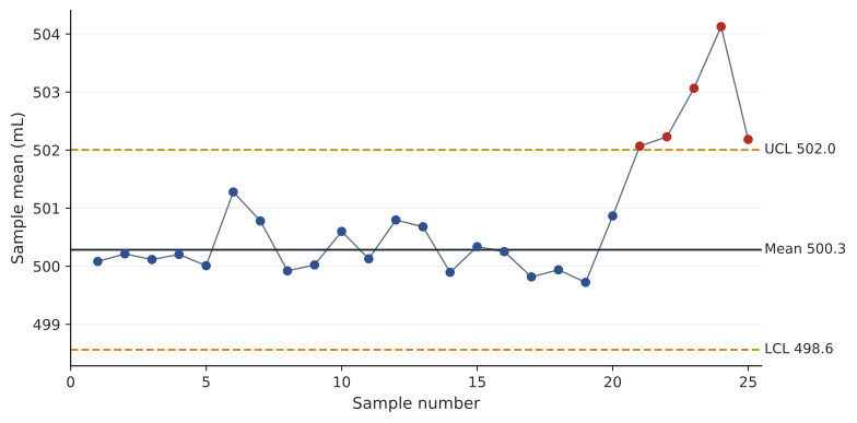
print(f"sigma {sigma:.2f} mL; Cp {cp:.2f}; Cpk {cpk:.2f}")Grand mean 500.28 mL, average range 2.98 mL x-bar chart: LCL 498.56 UCL 502.00; R chart: LCL 0.00 UCL 6.31 sample 18: mean 499.94 range 4.91 sample 19: mean 499.72 range 4.22 sample 20: mean 500.87 range 3.04 sample 21: mean 502.07 range 1.93 OUT sample 22: mean 502.23 range 2.47 OUT sample 23: mean 503.06 range 2.01 OUT sample 24: mean 504.13 range 2.09 OUT sample 25: mean 502.18 range 4.70 OUT sigma 1.28 mL; Cp 1.04; Cpk 0.97
The limits are set from the first 20 samples, when the filler was running normally. From sample 21, a simulated shift of 2 mL pushes every sample mean above the upper control limit, while the ranges stay normal: the filler is overfilling consistently rather than becoming erratic. In practice, an operator would stop and adjust the filler at the first signal. The last line of the output previews capability analysis, discussed below: even in control, this filler is only marginally capable of meeting a 496 to 504 mL specification.
Control charts for attributes
Attributes are characteristics that are counted rather than measured: a unit is defective or not, an invoice has an error or not, a call is resolved or not. For the proportion defective in samples of size \(n\), the p-chart is used. Its centre line is the average proportion defective \(\bar{p}\), and its limits are:
When the count of defects per unit is of interest, such as the number of scratches on a car door or the number of complaints per day, the c-chart is used, with centre line \(\bar{c}\) and limits \(\bar{c} \pm 3\sqrt{\bar{c}}\). Attribute charts need larger samples than variable charts because a yes-or-no observation carries less information than a measurement.
Worked problem
A p-chart for invoice errors
An accounts payable team audits 200 invoices each week. Over 12 weeks, it finds 96 invoices with errors in total. Calculate control limits for a p-chart. In week 13, 16 of 200 invoices contain errors. What should the team conclude?
Show solution
- p-bar = 96 ÷ (12 × 200) = 96 ÷ 2,400 = 0.04.
- Standard error = √(0.04 × 0.96 ÷ 200) = √0.000192 ≈ 0.01386.
- UCL = 0.04 + 3 × 0.01386 ≈ 0.0816; LCL = 0.04 − 0.0416 < 0, so LCL = 0.
- Week 13 proportion = 16 ÷ 200 = 0.08, just below the UCL of 0.0816.
- No out-of-control signal yet, but the point is close to the limit; the team should watch the next weeks and check for runs or trends.
Answer: The control limits are 0 and about 8.2 %. Week 13's 8 % error rate is unusually high but not beyond the limit, so the team should monitor closely rather than overreact.
Reading control charts
A point beyond the control limits is the clearest signal, but non-random patterns inside the limits also indicate special causes. Common rules, such as the Western Electric rules, flag a run of seven or eight consecutive points on one side of the centre line, six points in a row steadily increasing or decreasing, two of three consecutive points near a control limit, and cycles or other systematic patterns. Using too many rules at once raises the chance of false alarms, so organizations usually choose a few.
Control charts are most useful when they are kept by the people who run the process and acted on immediately. A control chart posted on a wall and updated weekly by a quality technician catches problems long after the defective product has been made. Modern sensors and software can chart thousands of variables automatically and alert operators in real time. Before charts are used for monitoring, the process must be brought into control, with special causes removed, and the limits calculated from that stable data. Limits should be recalculated after a deliberate process change.
Process capability
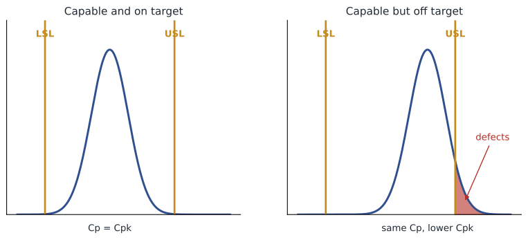
A process can be in statistical control and still produce many defects if its natural variation is too wide for the specification. Process capability compares the spread of the process with the specification limits set by the customer or designer. The capability ratio \(C_p\) compares the width of the specification with the natural spread of the process (six standard deviations). The capability index \(C_{pk}\) also accounts for whether the process is centred, using the distance from the mean to the nearer specification limit:
A \(C_p\) of 1.0 means the process spread exactly fills the specification, so even a perfectly centred process produces about 0.27 % defects (2,700 per million). Many firms require \(C_{pk}\) of at least 1.33 from their suppliers, and automotive and aerospace customers often require 1.67 for critical characteristics. If \(C_{pk}\) is much lower than \(C_p\), the process could be improved simply by centring it; if \(C_p\) itself is low, the process variation must be reduced.
Worked problem
Capability of a machining process
A bushing has a specified inside diameter of 20.00 ± 0.06 mm. The process is in control with a mean of 20.02 mm and a standard deviation of 0.012 mm. Calculate Cp and Cpk and interpret them.
Show solution
- USL = 20.06 mm; LSL = 19.94 mm; specification width = 0.12 mm.
- Cp = 0.12 ÷ (6 × 0.012) = 0.12 ÷ 0.072 ≈ 1.67.
- Distance to USL = 20.06 − 20.02 = 0.04; to LSL = 20.02 − 19.94 = 0.08.
- Cpk = min(0.04, 0.08) ÷ (3 × 0.012) = 0.04 ÷ 0.036 ≈ 1.11.
- The process is potentially very capable (Cp 1.67) but is off-centre toward the upper limit; recentring at 20.00 mm would raise Cpk to 1.67.
Answer: Cp is 1.67 but Cpk only 1.11. Adjusting the process to centre it on the target would make it fully capable without reducing variation.
Six Sigma
Six Sigma is a disciplined, data-driven approach to reducing variation and defects, developed at Motorola in the 1980s and popularized by General Electric in the 1990s. The name refers to a process whose specification limits lie six standard deviations from the mean. Allowing for a conventional long-term drift of 1.5 standard deviations in the process mean, a six sigma process produces about 3.4 defects per million opportunities (DPMO). A typical three sigma process, by the same convention, produces about 66,800 DPMO. Defects per million opportunities is calculated as:
| Sigma level (with 1.5σ shift) | Defects per million opportunities | Yield |
|---|---|---|
| 2 | 308,537 | 69.1 % |
| 3 | 66,807 | 93.3 % |
| 4 | 6,210 | 99.38 % |
| 5 | 233 | 99.977 % |
| 6 | 3.4 | 99.99966 % |
Worked problem
Calculating DPMO
A hospital pharmacy audits 2,500 medication orders. Each order has four opportunities for error (drug, dose, route and timing). The audit finds 30 errors. Calculate DPMO and the approximate sigma level.
Show solution
- Opportunities = 2,500 × 4 = 10,000.
- DPMO = 30 ÷ 10,000 × 1,000,000 = 3,000.
- From the table, 3,000 DPMO lies between 4 sigma (6,210) and 5 sigma (233), at roughly 4.2 sigma.
- Each error could harm a patient, so the pharmacy would aim much higher, using double checks, barcode scanning and error-proofing.
Answer: The pharmacy runs at about 3,000 DPMO, or roughly 4.2 sigma; for a safety-critical process, that is a strong case for improvement.
Six Sigma projects follow the DMAIC method. Define the problem, the customer requirements and the project scope, often in a project charter. Measure the current process performance and validate the measurement system. Analyze the data to find and verify root causes. Improve the process by developing, testing and implementing solutions. Control the improved process with control charts, standard work and monitoring so the gains last. For new processes or products, a related method, DMADV (define, measure, analyze, design, verify), is used.
Six Sigma also defines roles. Executive champions select projects aligned with strategy; Master Black Belts coach and train; Black Belts lead projects full time; Green Belts lead smaller projects alongside their regular jobs. Many organizations combine Six Sigma with lean (lesson 11) as Lean Six Sigma, using lean to remove waste and speed flow and Six Sigma to reduce variation. Critics note that Six Sigma can become bureaucratic and that the 3.4 DPMO target means little for processes where 'opportunities' are defined loosely; the underlying discipline of defining problems with data and verifying causes before acting is its lasting value.
Acceptance sampling
Acceptance sampling inspects a random sample from an incoming or outgoing lot and decides whether to accept or reject the whole lot. A sampling plan specifies the sample size and the maximum number of defectives allowed. An operating characteristic (OC) curve shows the probability of accepting lots of different quality levels under the plan. The producer's risk is the chance of rejecting a good lot (one at the acceptable quality level, or AQL); the consumer's risk is the chance of accepting a bad lot. Acceptance sampling is useful when inspecting every item is too costly or destructive, but it does nothing to improve quality, and modern practice shifts effort from inspecting lots to ensuring suppliers' processes are capable and in control.
Common mistakes
MistakeAdjusting a stable process every time a measurement moves.
InsteadDo not tamper; react only to control chart signals of special causes.
MistakeConfusing control limits with specification limits.
InsteadControl limits come from process data; specification limits come from customer requirements.
MistakeAssuming an in-control process is good enough.
InsteadCheck capability: a stable process can still produce many defects if Cp or Cpk is low.
MistakeLooking only at Cp.
InsteadUse Cpk as well, because an off-centre process produces more defects than Cp suggests.
MistakeSetting control limits from data that include special causes.
InsteadRemove special causes first, then calculate limits from stable data.
MistakeRelying on acceptance sampling to achieve quality.
InsteadBuild capable, controlled processes at the source; sampling only sorts lots.
Summary and key terms
- All processes vary; common causes are built in, special causes are specific events.
- A process with only common-cause variation is in statistical control; tampering with it adds variation.
- x-bar and R charts monitor the centre and spread of measured variables using constants A2, D3 and D4.
- p-charts monitor proportions defective; c-charts monitor counts of defects.
- Points outside the limits and non-random patterns signal special causes.
- Cp compares specification width with process spread; Cpk also accounts for centring.
- Many customers require Cpk of at least 1.33.
- Six Sigma targets 3.4 DPMO and uses the DMAIC method with trained project leaders.
- Acceptance sampling accepts or rejects lots but does not improve quality.
- Common cause
- A source of natural, random variation built into a process.
- Special cause
- A specific, identifiable source of unusual variation.
- Statistical control
- The state of a process with only common-cause variation.
- Control chart
- A chart plotting a sample statistic over time against control limits.
- x-bar chart
- A control chart of sample means that detects shifts in the process centre.
- R chart
- A control chart of sample ranges that detects changes in process spread.
- p-chart
- A control chart of the proportion defective in samples.
- Process capability
- The ability of a process to meet specification limits.
- DPMO
- Defects per million opportunities.
- DMAIC
- Define, measure, analyze, improve, control: the Six Sigma improvement method.
Practice problems
Work each problem on paper first, then reveal the answer to check.
Classify as common or special cause: normal temperature fluctuations; a broken tool.
Show answer
Common; special.
Sample size 4, grand mean 50, average range 2. Find the x-bar chart limits.
Show answer
50 ± 0.729 × 2 = 48.54 to 51.46.
For the same data, find the R chart UCL.
Show answer
2.282 × 2 = 4.56.
p-bar is 0.05 and n = 100. Find the UCL of the p-chart.
Show answer
0.05 + 3 × 0.0218 ≈ 0.115.
A c-chart has c-bar = 9. Find its limits.
Show answer
9 ± 9: LCL 0, UCL 18.
Specification 100 ± 3, σ = 0.5, mean 101. Find Cp and Cpk.
Show answer
Cp = 6 ÷ 3 = 2.0; Cpk = 2 ÷ 1.5 ≈ 1.33.
What does a run of eight points above the centre line suggest?
Show answer
A shift in the process mean, even if no point is outside the limits.
A firm inspects 500 units with 3 opportunities each and finds 6 defects. What is DPMO?
Show answer
6 ÷ 1,500 × 1,000,000 = 4,000.
Name the five DMAIC phases.
Show answer
Define, measure, analyze, improve, control.
Portfolio task: time a repeated activity (for example, your commute) for 20 days and plot an individuals chart.
Show answer
Answers vary; compute mean and limits and identify any special causes.
Lesson quiz · 5 questions
Score 60% or more to complete this lesson.
Create a free account to save your progress, take quizzes and earn a certificate.