Metapopulations, landscapes and connectivity

Few species live in a single continuous population. Most are spread across patches of habitat of varying size and quality, linked to a greater or lesser degree by the movement of individuals. Whether a species persists in a fragmented landscape depends not only on what happens within each patch but on how patches are connected. BIOL-208 introduced the Levins metapopulation model, sources and sinks, and the basic ideas of landscape fragmentation and corridors. This lesson applies those ideas to conservation: how habitat destruction pushes metapopulations toward an extinction threshold, how connectivity is measured and planned, and how corridors and wildlife crossings work in practice in Canada and the United States.

The metapopulation idea revisited

A metapopulation is a set of local populations occupying discrete habitat patches, connected by dispersal, in which local populations go extinct and patches are recolonized. Richard Levins's 1969 model, introduced in BIOL-208, tracks the fraction of patches occupied, \(p\), with a colonization rate \(c\) and a local extinction rate \(e\):

At equilibrium the fraction occupied is \(p^* = 1 - e/c\), and the metapopulation persists only if colonization exceeds extinction, \(c > e\). The model is a deliberate simplification: all patches are equal, every patch is equally reachable from every other, and local dynamics are ignored. Its value for conservation is the insight that a species can persist regionally even though every local population is doomed eventually, so long as empty patches are recolonized fast enough. It follows that protecting only currently occupied patches is not enough; unoccupied but suitable patches are part of the species' habitat, because they will be needed for future colonization.

Habitat destruction and the extinction threshold

Russell Lande, and later Sean Nee and Robert May in 1992, extended the Levins model to ask what happens when a fraction \(D\) of patches is permanently destroyed. Colonists landing on destroyed patches fail, so only the fraction \(1 - D - p\) of patches is available for colonization:

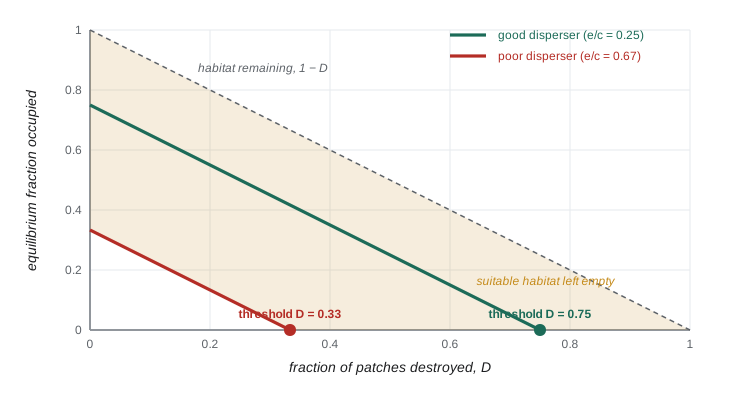
This simple result has three striking implications. First, occupancy falls one for one with habitat destroyed: each additional per cent of patches lost removes a per cent of occupied patches. Second, there is an extinction threshold: when \(D\) reaches \(1 - e/c\), occupancy falls to zero and the metapopulation goes extinct, even though suitable habitat remains, a fraction \(e/c\) of the original patches. A species can therefore disappear from a landscape that still contains apparently suitable but empty habitat. Third, the species most at risk are those with low colonization relative to extinction, typically poor dispersers, even if they are currently common. David Tilman and colleagues used a multispecies version of this model in 1994 to argue that habitat destruction leads to an extinction debt that falls disproportionately on the best competitors, which are often poor dispersers.

# Levins model with permanent destruction of a fraction D of patches.
# Two invented species with the same extinction rate but different colonization rates.
def simulate(c, e, D, p0=0.5, years=300, dt=0.1):
    p = p0
    for _ in range(int(years / dt)):
        p += dt * (c * p * (1 - D - p) - e * p)
        p = max(p, 0.0)
    return p
e = 0.2
for name, c in (("good disperser", 0.8), ("poor disperser", 0.3)):
    thresh = 1 - e / c
    print(f"{name}: c = {c}, e = {e}, extinction threshold D* = {thresh:.2f}")
    for D in (0.0, 0.2, 0.4, 0.6, 0.7):
        print(f"   D = {D:.1f}: occupancy after 300 years = {simulate(c, e, D):.3f}  (theory {max(1 - D - e / c, 0):.3f})")

good disperser: c = 0.8, e = 0.2, extinction threshold D* = 0.75
   D = 0.0: occupancy after 300 years = 0.750  (theory 0.750)
   D = 0.2: occupancy after 300 years = 0.550  (theory 0.550)
   D = 0.4: occupancy after 300 years = 0.350  (theory 0.350)
   D = 0.6: occupancy after 300 years = 0.150  (theory 0.150)
   D = 0.7: occupancy after 300 years = 0.050  (theory 0.050)
poor disperser: c = 0.3, e = 0.2, extinction threshold D* = 0.33
   D = 0.0: occupancy after 300 years = 0.333  (theory 0.333)
   D = 0.2: occupancy after 300 years = 0.133  (theory 0.133)
   D = 0.4: occupancy after 300 years = 0.000  (theory 0.000)
   D = 0.6: occupancy after 300 years = 0.000  (theory 0.000)
   D = 0.7: occupancy after 300 years = 0.000  (theory 0.000)

The good disperser persists until about three quarters of its patches are destroyed, while the poor disperser, with the same local extinction rate, disappears once about a third are destroyed. At D = 0.4 the poor disperser is already gone even though 60 per cent of its patches remain. In real landscapes the threshold depends on the spatial arrangement of patches as well as their number, and spatially explicit models typically show thresholds that are reached sooner than the simple model predicts, because destroyed patches are usually clustered and remaining patches become isolated.

Beyond the Levins model

Real metapopulations differ from the Levins ideal in ways that matter for conservation. Ilkka Hanski's long-term studies of the Glanville fritillary butterfly in the Åland Islands of Finland, which occupies several thousand small meadows, showed that colonization depends on the distance to occupied patches and extinction depends on patch area. His incidence function model, published in 1994, uses these relationships to predict which patches are likely to be occupied and has been applied to many species. Large patches with low extinction risk can act as mainlands that supply colonists to smaller ones, a structure called a mainland–island or core–satellite metapopulation. Sources and sinks, introduced in BIOL-208, add another twist: a high-quality source patch may support sink patches that would be empty on their own, so destroying a source can eliminate several sinks.

These refinements lead to practical rules. Large patches are especially valuable because they persist longest and supply colonists. Patches that are close to other occupied patches are more likely to be recolonized. And the matrix between patches matters: a hedgerow or a forested stream bank may allow movement across farmland that open fields would block.

Landscape connectivity

Connectivity is the degree to which a landscape facilitates or impedes the movement of organisms among resource patches, as defined by Philip Taylor and colleagues in 1993. Structural connectivity describes the physical arrangement of habitat, such as whether patches touch or are joined by strips of habitat. Functional connectivity describes how a particular species actually moves: a strip of trees may connect forest patches for a squirrel but not for a forest-interior songbird that avoids edges, and a two-lane road may be a minor obstacle for a deer but a lethal barrier for a turtle. Because functional connectivity is species-specific, conservation planners often model connectivity for several focal species with different requirements.

Two families of methods dominate connectivity modelling. Both start with a resistance surface, a map in which each cell is assigned a cost of movement for the species of interest, based on land cover, roads, terrain and human activity, often estimated from telemetry or genetic data. Least-cost path analysis finds the route between two habitat patches with the lowest cumulative resistance, using shortest-path algorithms from computer science such as Dijkstra's algorithm. Circuit theory, introduced to ecology by Brad McRae in 2006 and implemented in the widely used software Circuitscape, treats the landscape as an electrical circuit in which current flows between patches through all possible paths; areas where current is concentrated are pinch points, where loss of habitat would most reduce connectivity. Least-cost paths identify the single best route, while circuit theory shows where movement is spread and where it is funnelled.

import heapq
# Least-cost path across an invented resistance grid with Dijkstra's algorithm.
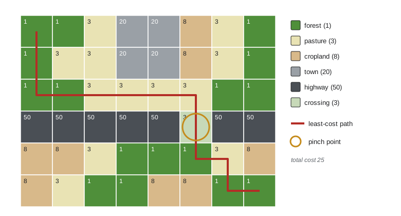
# 1 = forest, 3 = pasture, 8 = cropland, 50 = highway, 20 = town; start at top-left, end at bottom-right.
grid = [
    [1, 1, 3, 20, 20, 8, 3, 1],
    [1, 3, 3, 20, 20, 8, 3, 1],
    [1, 1, 3, 3, 3, 3, 1, 1],
    [50, 50, 50, 50, 50, 3, 50, 50],
    [8, 8, 3, 1, 1, 1, 3, 8],
    [8, 3, 1, 1, 8, 8, 1, 1],
]
rows, cols = len(grid), len(grid[0])
start, goal = (0, 0), (rows - 1, cols - 1)
dist = {start: grid[0][0]}; prev = {}; heap = [(grid[0][0], start)]
while heap:
    d, (r, c) = heapq.heappop(heap)
    if (r, c) == goal: break
    if d > dist[(r, c)]: continue
    for dr, dc in ((1, 0), (-1, 0), (0, 1), (0, -1)):
        nr, nc = r + dr, c + dc
        if 0 <= nr < rows and 0 <= nc < cols:
            nd = d + grid[nr][nc]
            if nd < dist.get((nr, nc), float("inf")):
                dist[(nr, nc)] = nd; prev[(nr, nc)] = (r, c); heapq.heappush(heap, (nd, (nr, nc)))
path, node = [goal], goal
while node != start:
    node = prev[node]; path.append(node)
path.reverse()
print("least-cost path:", " ".join(f"{r}{c}" for r, c in path))
print("cumulative cost:", dist[goal])
print("highway crossed at row 3, column", [c for r, c in path if r == 3])
for r in range(rows):
    print(" ".join("*" if (r, c) in path else "." for c in range(cols)))

least-cost path: 00 10 20 21 22 23 24 25 35 45 46 56 57
cumulative cost: 25
highway crossed at row 3, column [5]
* . . . . . . .
* . . . . . . .
* * * * * * . .
. . . . . * . .
. . . . . * * .
. . . . . . * *

The least-cost path finds the one cell in the highway row where resistance is low, an underpass or a bridge over a creek, and routes through it, avoiding the town and most of the cropland. In planning terms, that cell is a pinch point: if it were blocked, the cost of movement would rise sharply. Real analyses use grids of millions of cells and resistance values estimated from data, and they test how sensitive the results are to the assumed resistances, which are often the weakest part of the analysis.

Do corridors work?

A corridor is a strip of habitat that connects otherwise isolated patches. Corridors were proposed in the 1970s and 1980s as a way to apply island biogeography to reserve design, and they were debated vigorously in the 1990s, when critics such as Daniel Simberloff pointed out that corridors are costly, that evidence of their benefits was thin, and that they might spread disease, fire or invasive species. Since then experimental and observational evidence has accumulated. Large-scale experiments at the Savannah River Site in South Carolina, begun in the 1990s by Nick Haddad, Doug Levey, Joshua Tewksbury and colleagues, created patches of open pine habitat connected or not connected by corridors; they found that corridors increased movement of butterflies, birds and seeds between patches, increased pollination and seed dispersal, and increased plant species richness over time. A 2010 meta-analysis by Lindsay Gilbert-Norton and colleagues found that corridors increased movement between patches by about 50 per cent compared with unconnected patches. Corridors are now widely accepted as useful, with the caveat that their design must fit the species that are meant to use them.

Connectivity at continental and local scales

At the largest scale, the Yellowstone to Yukon Conservation Initiative, launched in 1993, aims to maintain connectivity along about 3,200 kilometres of the Rocky Mountains from Wyoming to the Yukon, so that wide-ranging species such as grizzly bears, wolves, wolverines and elk can move through a network of protected areas and compatible working lands. The idea was inspired partly by a wolf named Pluie, fitted with a satellite collar in Alberta in 1991, which travelled over an area of about 100,000 square kilometres across two countries, two provinces and three states before being shot. Large-landscape connectivity projects now exist in many regions, including the Algonquin to Adirondacks initiative linking Ontario and New York.

At local scales, wildlife crossing structures allow animals to pass over or under roads. Banff National Park in Alberta has one of the world's best-studied systems: since the 1980s the twinning of the Trans-Canada Highway through the park has been accompanied by wildlife fencing and dozens of underpasses and overpasses. Long-term monitoring led by Tony Clevenger and colleagues documented hundreds of thousands of crossings by animals including grizzly and black bears, wolves, cougars, elk and deer, and showed that fencing and crossings reduced collisions between vehicles and large animals by more than 80 per cent. Genetic studies found that grizzly and black bears on either side of the highway were interbreeding through the crossings, so the structures were restoring gene flow, not only movement. In the United States, the Infrastructure Investment and Jobs Act of 2021 created a Wildlife Crossings Pilot Program with 350 million US dollars over five years, and states such as Colorado, Utah, Wyoming and California have built major crossings; the Wallis Annenberg Wildlife Crossing over a ten-lane freeway near Los Angeles, intended to reconnect a small, isolated population of mountain lions, is among the largest.

Connectivity for a changing climate

Climate change adds urgency to connectivity. As climates shift, species must move to track suitable conditions, and in fragmented landscapes many will be unable to do so. Planners are therefore designing connectivity networks that link current habitat to areas expected to be suitable in future, that follow gradients of temperature and moisture, and that protect climate refugia, places such as north-facing slopes, cold-air pockets and groundwater-fed streams where conditions are expected to change more slowly. Riparian corridors along rivers are particularly valuable because they cross temperature gradients and provide water and shade. Lesson 8 shows how connectivity is incorporated into systematic conservation planning.