
BIOL-367 · Lesson 2 of 12 · 27 min
Measuring biodiversity
Before biodiversity can be protected it has to be described, and before it can be described it has to be counted. Counting turns out to be surprisingly difficult. Most species are small, rare or hard to find, the number of species found in a survey depends on how hard you look, and different measures of diversity can rank the same places in different orders. BIOL-208 introduced species richness, the Shannon and Simpson indices and beta diversity for describing communities. This lesson builds on that foundation with the tools conservation biologists use to compare places fairly, to estimate how many species are present but unseen, to relate species numbers to area, and to identify places and species that deserve priority.
What exactly are we counting?
Most biodiversity measurement focuses on species, but species counts can hide important differences. Two forests may each contain 40 tree species, yet in one forest a single species makes up 90 per cent of the trees, while in the other the trees are evenly spread among species. Two lakes may each hold ten fish species, but in one lake all ten are closely related minnows while the other holds a sturgeon, a gar, a lamprey and several other ancient lineages. And two grasslands may have similar species lists but very different ecological functions if one has lost its large grazers and burrowing mammals. For these reasons conservation biologists use several complementary measures.
Genetic diversity is usually measured within species as heterozygosity, allelic richness or nucleotide diversity, as described in BIOL-322. It matters because populations need genetic variation to adapt to changing conditions, and because loss of variation through drift and inbreeding can reduce fitness. The Kunming–Montreal Global Biodiversity Framework adopted in 2022 includes a target to maintain the genetic diversity of wild and domesticated species, and one widely discussed indicator is the proportion of populations with an effective size above 500.
Functional diversity measures the range of traits and ecological roles in a community, such as body size, diet, rooting depth or nitrogen fixation. Communities with high functional diversity often process energy and nutrients more completely and are more resistant to disturbance, because when one species declines, another with similar traits can take over. Phylogenetic diversity, defined by Daniel Faith in 1992 as the total branch length of the evolutionary tree connecting a set of species, measures how much evolutionary history a community contains. Protecting a species that is the only survivor of an ancient lineage, such as the tuatara of New Zealand or the paddlefish of the Mississippi basin, conserves more evolutionary history than protecting one of many close relatives. The EDGE of Existence program of the Zoological Society of London ranks species by combining evolutionary distinctiveness with global endangerment.
Hill numbers: diversity as an effective number of species
The Shannon and Simpson indices described in BIOL-208 are useful but awkward to interpret: a Shannon index of 2.3 does not tell you directly how diverse a community is, and a doubling of the index does not mean a doubling of diversity. Ecologists now commonly convert these indices into Hill numbers, named for the ecologist Mark Hill, who proposed them in 1973. A Hill number of order \(q\) gives the effective number of equally common species that would produce the observed value of an index:
Here \(p_i\) is the proportion of individuals belonging to species \(i\) and \(S\) is the number of species. The order \(q\) controls how much weight is given to common versus rare species. When \(q = 0\), every species counts equally and \({}^0D\) is simply species richness. When \(q = 1\), the formula is undefined but its limit is the exponential of the Shannon index, \({}^1D = \exp(H')\), which weights species in proportion to their abundance. When \(q = 2\), \({}^2D\) is the inverse of the Simpson concentration \(\sum p_i^2\), which emphasizes the dominant species. For any community, \({}^0D \ge {}^1D \ge {}^2D\), and the three are equal only if all species are equally abundant.
Hill numbers have two great advantages. They are all expressed in the same unit, species, so they can be compared directly and plotted together as a diversity profile. And they obey the doubling property: if two communities with no species in common and the same diversity are pooled in equal amounts, the Hill number of the pooled community is twice that of each original. A community with \({}^1D\) of 20 is twice as diverse, in this sense, as one with \({}^1D\) of 10. For these reasons Hill numbers are increasingly recommended for biodiversity monitoring.
Sampling effort and rarefaction
The number of species recorded in a survey almost always increases with sampling effort. A first hour of netting in a pond catches the common species; later hours add rarer ones; and some species may never be caught at all. Plotting the cumulative number of species against the number of individuals or samples gives a species accumulation curve, which rises steeply at first and then flattens. If two sites are sampled with different effort, comparing their raw species counts is unfair: the site sampled more intensively will usually appear richer.
Rarefaction solves this problem by asking how many species would be expected if every site were sampled down to the same number of individuals. If a sample contains \(N\) individuals in \(S\) species, with \(N_i\) individuals of species \(i\), the expected number of species in a random subsample of \(n\) individuals drawn without replacement is
Each term is the probability that species \(i\) appears at least once in the subsample. Rarefaction curves for different sites can then be compared at the size of the smallest sample. Rarefaction discards information, however, and modern practice often extrapolates the curves forward as well, using the methods of Anne Chao and colleagues, so that sites can be compared at a common level of sample completeness rather than a common sample size.
Estimating species you have not seen
Even a well-sampled site usually contains species that were not detected. Anne Chao proposed in 1984 a simple estimator of the minimum true richness that uses the number of rare species in the sample. If \(f_1\) is the number of singletons, species represented by exactly one individual, and \(f_2\) is the number of doubletons, species represented by exactly two, then the Chao1 estimator is
The logic is that if many species appear only once, many others probably have not yet appeared at all; if most species have been seen several times, the inventory is nearly complete. A related quantity, sample coverage, estimates the proportion of the community's individuals that belong to species already detected. It is approximately \(1 - f_1/N\), so a sample of 500 individuals with 10 singletons has a coverage of about 98 per cent. Chao1 is a lower bound, not an exact estimate, and it works best when sampling is random and species are not extremely clumped.
import math
# Invented counts of beetles in pitfall traps at two prairie sites (individuals per species).
site_a = [52, 31, 22, 15, 11, 9, 7, 6, 4, 3, 3, 2, 2, 1, 1, 1, 1, 1]
site_b = [120, 64, 40, 28, 18, 12, 9, 7, 5, 4, 3, 3, 2, 2, 2, 1, 1, 1, 1, 1, 1, 1, 1, 1]

def hill(counts, q):
    n = sum(counts); p = [c / n for c in counts]
    if q == 1:
        return math.exp(-sum(x * math.log(x) for x in p))
    return sum(x ** q for x in p) ** (1 / (1 - q))

def rarefy(counts, m):
    n = sum(counts)
    return sum(1 - math.comb(n - c, m) / math.comb(n, m) for c in counts)

def chao1(counts):
    f1 = counts.count(1); f2 = counts.count(2)
    return len(counts) + (f1 * f1 / (2 * f2) if f2 else f1 * (f1 - 1) / 2)

for name, c in (("A", site_a), ("B", site_b)):
    n = sum(c)
    print(f"site {name}: N = {n:3d}, observed S = {len(c):2d}, 1D = {hill(c, 1):5.2f}, "
          f"2D = {hill(c, 2):5.2f}, Chao1 = {chao1(c):5.1f}, coverage = {1 - c.count(1) / n:.3f}")
m = min(sum(site_a), sum(site_b))
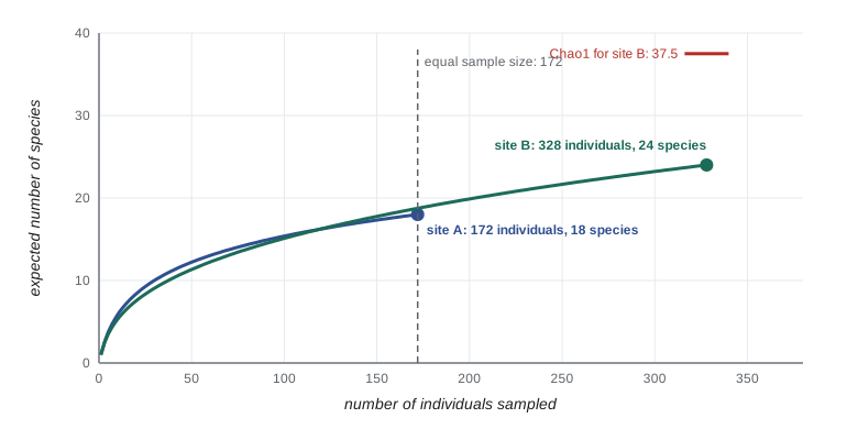
print(f"rarefied to {m} individuals: A = {rarefy(site_a, m):.1f} species, B = {rarefy(site_b, m):.1f} species")site A: N = 172, observed S = 18, 1D = 9.08, 2D = 6.28, Chao1 = 24.2, coverage = 0.971 site B: N = 328, observed S = 24, 1D = 7.93, 2D = 4.99, Chao1 = 37.5, coverage = 0.973 rarefied to 172 individuals: A = 18.0 species, B = 18.8 species
Site B appears richer in raw numbers because it was sampled more heavily, with more than twice as many individuals. Rarefied to the size of site A's sample, its expected richness is much closer to site A's, and its Hill numbers of order 1 and 2 show that its community is dominated more strongly by a few abundant species. Site B also has many singletons, so its Chao1 estimate is well above the observed count: more sampling would probably find more species there. A careless comparison of raw counts would have reached the wrong conclusion.
How many species are there?
About 2.1 million species have been formally described, but the true number on Earth is far larger. Estimates for eukaryotes alone range from about 2 million to more than 10 million; a frequently cited 2011 study by Camilo Mora and colleagues estimated about 8.7 million eukaryotic species, of which more than 80 per cent remain undescribed. Estimates for bacteria and archaea are far more uncertain and run into the billions, depending on how species are defined. Insects, fungi, nematodes and mites make up most of the undescribed eukaryotes, and most of them live in tropical forests, soils and the deep sea.
For conservation this matters in two ways. First, most extinctions are probably occurring among species that have never been named, so documented extinctions are a large underestimate of real losses. Second, conservation cannot wait for complete inventories, so it relies on surrogates: well-known groups such as birds, mammals, butterflies or vascular plants are used to stand in for the rest. Surrogates work only if patterns of diversity in different groups coincide, which they often do at broad scales but less reliably at fine scales.
The species–area relationship
One of the oldest generalizations in ecology is that larger areas contain more species. The relationship is usually described by a power function first used systematically by Olof Arrhenius in 1921:
Here \(S\) is the number of species, \(A\) is area, \(c\) is a constant that depends on the group and region, and \(z\) is the slope on a log–log plot. For nested samples within continuous habitat, \(z\) is typically about 0.1 to 0.2; for islands or isolated habitat fragments it is typically about 0.25 to 0.35, because isolated areas receive fewer immigrants. A useful rule of thumb follows from \(z \approx 0.25\): a tenfold increase in area roughly doubles the number of species, since \(10^{0.25} \approx 1.8\). The relationship arises because larger areas contain more individuals, more habitat types and larger populations that are less likely to go extinct, as island biogeography theory explains. Lesson 4 uses the species–area relationship in reverse, to estimate how many species may be lost when habitat is destroyed.
Rarity
Most species in most communities are rare, and rarity is a major predictor of extinction risk. But rarity has several dimensions. In 1981 Deborah Rabinowitz classified species by three traits: whether their geographic range is large or small, whether their habitat specificity is broad or narrow, and whether their local populations are large or small. Of the eight combinations, one describes common species, with large ranges, broad habitat tolerance and large local populations; the other seven are different forms of rarity. A species such as the Vancouver Island marmot, restricted to a small range, a narrow habitat of subalpine meadows and small local colonies, is rare in all three senses and is especially vulnerable. A species such as the peregrine falcon, with a worldwide range and broad habitat use but small local populations, is rare in only one sense.
| Range | Habitat specificity | Local population | Example of the pattern |
|---|---|---|---|
| Large | Broad | Large | Common: American robin |
| Large | Broad | Small | Sparse everywhere: peregrine falcon |
| Large | Narrow | Large | Habitat specialist but locally abundant: some salt-marsh plants |
| Small | Broad | Large | Narrow range but common within it: many island species |
| Small | Narrow | Small | Rare in every sense: Vancouver Island marmot |
Endemism is closely related to range size. A species is endemic to a region if it occurs nowhere else. Endemic species with small ranges are vulnerable because a single disturbance, such as a dam, a new invasive predator or a development, can affect their entire range. Canada has relatively few endemic species compared with tropical countries, because most of its territory was covered by ice until about 10,000 to 15,000 years ago and was recolonized from the south; notable endemics include the Banff Springs snail, found only in a few hot springs in Banff National Park, and plants of the Gulf of St. Lawrence and the unglaciated refugia of the Yukon. The United States has many more endemics, especially in Hawaii, California, the southern Appalachians and the springs and caves of the arid Southwest.
Hotspots and priority places
Because conservation resources are limited, many organizations have tried to identify places where action would protect the most biodiversity. In 1988 Norman Myers proposed the idea of biodiversity hotspots, and in 2000 Myers and colleagues defined them as regions with at least 1,500 endemic vascular plant species that have lost at least 70 per cent of their original habitat. The original 25 hotspots covered only about 1.4 per cent of the land surface but held about 44 per cent of vascular plant species and 35 per cent of terrestrial vertebrate species as endemics. The list has since grown to 36, including the California Floristic Province and, since 2016, the North American Coastal Plain, which stretches from Texas to Massachusetts.
Hotspots are one priority-setting scheme among several. Others emphasize the opposite end of the spectrum: high-biodiversity wilderness areas, such as the boreal forest and the Amazon, that remain largely intact and can still be protected at large scales before they are degraded. Others focus on ecoregions, key biodiversity areas identified by a global standard published by the IUCN in 2016, or important bird and biodiversity areas. Each scheme uses different criteria, and lesson 8 shows how systematic conservation planning combines them using the principle of complementarity.
Worked problem
Comparing three wetlands with Hill numbers
Three wetlands each contain six waterbird species. Their proportions are: wetland 1, all six species at 1/6 each; wetland 2, 0.5, 0.3, 0.1, 0.05, 0.03 and 0.02; wetland 3, 0.9 and 0.02 for each of the other five. Rank the wetlands by richness and by the inverse Simpson index, the Hill number of order 2.
Show solution
- Richness, the Hill number of order 0, is 6 for all three wetlands, so richness alone cannot separate them.
- For wetland 1, \(\sum p_i^2 = 6 \times (1/6)^2 = 1/6\), so \({}^2D = 6\).
- For wetland 2, \(\sum p_i^2 = 0.25 + 0.09 + 0.01 + 0.0025 + 0.0009 + 0.0004 = 0.3538\), so \({}^2D \approx 2.8\).
- For wetland 3, \(\sum p_i^2 = 0.81 + 5 \times 0.0004 = 0.812\), so \({}^2D \approx 1.2\).
Answer: The order is wetland 1, then 2, then 3. Wetland 3 behaves almost like a one-species community because a single bird dominates it, even though six species are present.
Common mistakes
MistakeComparing raw species counts between sites sampled with different effort.
InsteadUse rarefaction or coverage-based comparisons so that sites are compared at equal sample size or completeness.
MistakeTreating the Shannon index as if it were a number of species.
InsteadConvert it to a Hill number, exp(H'), which is an effective number of species.
MistakeTreating Chao1 as an exact count of species.
InsteadIt is an estimated lower bound and depends on random sampling.
MistakeAssuming z in the species–area relationship is the same everywhere.
InsteadIt is usually lower for nested samples of continuous habitat and higher for islands and isolated fragments.
MistakeUsing one definition of rarity.
InsteadRarity can involve small range, narrow habitat or small local populations, and the combination matters for risk.
Summary and key terms
- Biodiversity can be measured as genetic, species, functional and phylogenetic diversity, each capturing different information.
- Hill numbers express diversity as an effective number of species; order 0 is richness, order 1 is exp(H') and order 2 is inverse Simpson.
- Species counts depend on sampling effort; rarefaction and coverage-based methods allow fair comparison.
- Chao1 uses singletons and doubletons to estimate the minimum number of species including those not detected.
- About 2.1 million species are described; the true number of eukaryotes is probably several times larger.
- The species–area relationship S = cA^z has z of about 0.1 to 0.2 within continuous habitat and 0.25 to 0.35 for islands.
- Rarity has dimensions of range, habitat specificity and local abundance; hotspots and other schemes help set priorities.
- Hill number
- An effective number of equally common species corresponding to a diversity index of order q.
- species accumulation curve
- A plot of cumulative species recorded against sampling effort.
- rarefaction
- Estimating expected species richness at a smaller standard sample size.
- Chao1
- An estimator of minimum species richness based on numbers of singletons and doubletons.
- sample coverage
- The estimated proportion of individuals in a community that belong to detected species.
- phylogenetic diversity
- The total branch length of the evolutionary tree linking a set of species.
- functional diversity
- The variety of traits and ecological roles among species in a community.
- species–area relationship
- The increase in species number with area, often S = cA^z.
- endemic
- Found naturally in only one region.
- biodiversity hotspot
- A region with at least 1,500 endemic plant species that has lost at least 70 per cent of its habitat.
- surrogate
- A well-known group or measure used to represent biodiversity that cannot be measured directly.
Practice problems
Work each problem on paper first, then reveal the answer to check.
What are the Hill numbers of order 0, 1 and 2?
Show answer
Species richness, the exponential of the Shannon index, and the inverse of the Simpson concentration.
Why should sites be rarefied before comparing richness?
Show answer
Because richness increases with sampling effort, so unequal samples bias comparisons.
A sample has 30 species, 8 singletons and 4 doubletons. What is Chao1?
Show answer
30 + 64/8 = 38 species.
Estimate coverage for 400 individuals with 8 singletons.
Show answer
About 1 − 8/400 = 0.98.
If z = 0.25, how much does richness increase when area increases a hundredfold?
Show answer
By 100^0.25 ≈ 3.2 times.
Why is z usually higher for islands than for nested samples?
Show answer
Isolated areas receive fewer immigrants, so small islands lose proportionally more species.
Name the three axes of Rabinowitz's rarity scheme.
Show answer
Geographic range, habitat specificity and local population size.
What two criteria define a biodiversity hotspot?
Show answer
At least 1,500 endemic vascular plants and at least 70 per cent habitat loss.
Lesson quiz · 5 questions
Score 60% or more to complete this lesson.
Create a free account to save your progress, take quizzes and earn a certificate.