
BIOL-330 · Lesson 3 of 12 · 33 min
Microbial growth and its measurement
In microbiology, growth means an increase in the number of cells rather than in the size of an individual. Most bacteria and archaea reproduce by binary fission: a cell enlarges, replicates its chromosome, segregates the copies to opposite halves and divides through the middle by constricting an FtsZ ring. Some bacteria bud, some fragment, and Streptomyces grows as branching filaments before forming spores, but the arithmetic of binary fission underlies almost every growth calculation. This lesson develops that arithmetic, describes how cell numbers are measured in practice, and follows a population through the phases of batch culture and into the steady state of continuous culture. Population growth in ecology, with logistic curves and carrying capacity, was treated in BIOL-208; here the emphasis is on laboratory measurement and the physiology behind the curves.
Exponential growth
If every cell divides into two after a fixed interval, the number of cells doubles in each generation. After n generations, a population that started with N₀ cells has:
Taking logarithms gives n = (log N − log N₀)/log 2, which is the form used to count generations from measured cell numbers. Dividing the elapsed time t by n gives the generation time (or doubling time) g, and its reciprocal, the number of generations per hour, is called the growth rate constant k. Microbiologists also use the specific growth rate μ, the rate constant of the continuous exponential equation dN/dt = μN, so that N = N₀e^{μt}. The two are related simply:
Generation times vary enormously. E. coli in rich medium at 37 °C doubles about every 20 minutes, the marine bacterium Vibrio natriegens in under 10 minutes, Mycobacterium tuberculosis every 15 to 20 hours, and some deep-subsurface communities apparently once in decades or centuries. Fast growers seem to defy arithmetic: replicating the 4.6-million-base E. coli chromosome takes about 40 minutes, longer than the 20-minute doubling time. The solution is multifork replication: a new round of replication begins before the previous one has finished, so rapidly growing cells contain several partly replicated chromosomes and each daughter inherits a chromosome that is already being copied.
Exponential growth cannot last. A single E. coli cell of about 10⁻¹² g doubling every 20 minutes would, if growth continued unchecked for two days, produce a mass thousands of times that of Earth. In reality, nutrients run out, wastes accumulate and growth stops. The useful idea is that exponential growth is what cells do when nothing is limiting, and for a few hours in the laboratory that is exactly what happens.
Worked problem
Generation time from plate counts
A culture contains 3.0 × 10⁴ cells per mL at 9:00 and 6.0 × 10⁷ cells per mL at 13:00, and was in exponential phase throughout. Find the number of generations, the generation time and μ.
Show solution
- n = (log 6.0 × 10⁷ − log 3.0 × 10⁴)/log 2 = (7.778 − 4.477)/0.301 = 10.97 generations.
- The elapsed time is 240 minutes, so g = 240/10.97 ≈ 21.9 minutes.
- μ = ln 2/g = 0.693/0.365 h ≈ 1.90 per hour.
Answer: About 11 generations, a generation time of about 22 minutes and μ ≈ 1.9 per hour, typical of E. coli in rich medium.
Counting cells: total counts
Lesson 1 showed how to count cells directly in a counting chamber. Total counts can also be made automatically. Electronic particle counters such as the Coulter counter detect the change in electrical resistance as each cell passes through a small aperture, and flow cytometers pass cells single file through a laser beam and record their light scatter and fluorescence, counting thousands of cells per second. Flow cytometry with live/dead dyes or fluorescent reporters can count particular subpopulations, and it has become the standard method for counting marine picoplankton. Total counts include dead cells, so they overestimate the number of cells able to grow.
Counting cells: viable counts and serial dilution
A viable count measures the cells able to divide and form colonies. Because a dense culture may contain 10⁹ cells per mL and a plate can show only a few hundred separate colonies, the sample must first be diluted by a known factor. In serial dilution, a small volume is transferred into a larger volume of sterile diluent, mixed and transferred again, so that each step multiplies the dilution. Ten-fold steps of 1 mL into 9 mL are most common. A known volume of each dilution is then spread on a plate or mixed with molten agar in a pour plate, and the colonies are counted after incubation.
Only plates within a countable range are used, usually 30 to 300 colonies for a standard Petri dish (25 to 250 in some food and water methods). Below the range, Poisson counting error is large; above it, colonies merge and compete. Because some colonies arise from pairs, chains or clumps of cells rather than single cells, results are reported in colony-forming units (CFU) rather than cells. The concentration in the original sample is:
where the dilution is written as a fraction, such as 10⁻⁶. Equivalently, multiply the colony count by the reciprocal of the dilution and divide by the volume plated.
import numpy as np

rng = np.random.default_rng(330)
true_cfu_per_mL = 1.5e9
dilutions = [1e-4, 1e-5, 1e-6, 1e-7]
vol_plated = 0.1                                 # mL spread on each plate
print("dilution  plate A  plate B   usable?")
usable = []
for d in dilutions:
    expected = true_cfu_per_mL * d * vol_plated
    a, b = rng.poisson(expected, 2)
    ok = all(30 <= c <= 300 for c in (a, b))
    flag = "yes" if ok else ("TNTC" if min(a, b) > 300 else "too few")
    print(f"{d:8.0e}  {a:7d}  {b:7d}   {flag}")
    if ok:
        usable.append((d, (a + b) / 2))
for d, mean in usable:
    est = mean / (vol_plated * d)
    se = np.sqrt(2 * mean) / 2 / (vol_plated * d)
print(f"estimate from {d:.0e}: {est:.3g} CFU/mL (SE about {se:.2g})")dilution plate A plate B usable? 1e-04 15129 15147 TNTC 1e-05 1459 1423 TNTC 1e-06 98 147 yes 1e-07 13 15 too few estimate from 1e-06: 1.22e+09 CFU/mL (SE about 7.8e+07)
The simulation reproduces what happens on the bench. The 10⁻⁴ and 10⁻⁵ plates are too numerous to count (TNTC), the 10⁻⁷ plates have too few colonies to be reliable, and the duplicate 10⁻⁶ plates fall in the countable range. Their estimate, 1.2 × 10⁹ CFU per mL, is within about 20 per cent of the true value used in the simulation (1.5 × 10⁹), even though the Poisson standard error is only about 6 per cent: the two plates happened to differ more than average, a reminder that one or two plates give a rough estimate. In real work, pipetting error at each dilution step adds to the counting error, so a series of six ten-fold dilutions can easily carry an overall uncertainty of 10 to 20 per cent. Microbiologists therefore report counts to two significant figures and think in logarithms: a difference between 1.4 × 10⁹ and 1.6 × 10⁹ CFU per mL is noise, but a difference of one log unit is real.
Viable counts have their own blind spots. They count only organisms that grow on the chosen medium under the chosen conditions, which, as lesson 1 showed, may be a small fraction of environmental cells. Stressed cells, such as those injured by freezing or mild heat in food processing, may survive but fail to form colonies on selective media, so food methods often include a resuscitation step on non-selective medium. Some pathogens, including Vibrio cholerae and Campylobacter, can enter a viable but non-culturable state in which they keep metabolizing but do not form colonies.
Most probable number
When cell concentrations are very low, or when an organism is recognized more easily by what it does in liquid than by its colonies, the most probable number (MPN) method is used. Several tubes of medium are inoculated at each of three or more dilutions, incubated, and scored for growth or a characteristic reaction, such as gas from lactose in coliform tests. The logic is statistical: a tube is positive if it received at least one viable cell, and the probability of receiving none at a mean concentration λ per tube is e^{−λ} from the Poisson distribution. The MPN is the concentration that makes the observed pattern of positive and negative tubes most likely. Published tables give the answer for standard designs, and it can also be computed directly, as below. MPN methods are less precise than plate counts, but they are still widely used for water, shellfish and food testing.
import numpy as np
from scipy.optimize import minimize_scalar

# Three dilutions, five tubes each: volumes of original sample per tube (mL)
volumes = np.array([10.0, 1.0, 0.1])
n_tubes = np.array([5, 5, 5])
positive = np.array([5, 3, 0])          # observed positive tubes

def neg_log_lik(log_c):
    c = np.exp(log_c)                     # organisms per mL
    p_pos = 1 - np.exp(-c * volumes)      # P(tube receives >= 1 organism)
    p_pos = np.clip(p_pos, 1e-12, 1 - 1e-12)
    return -np.sum(positive * np.log(p_pos) + (n_tubes - positive) * np.log(1 - p_pos))

res = minimize_scalar(neg_log_lik, bounds=(np.log(1e-3), np.log(1e3)), method="bounded")
mpn = np.exp(res.x)
print(f"MPN = {mpn:.2f} organisms per mL = {100*mpn:.0f} per 100 mL")MPN = 0.79 organisms per mL = 79 per 100 mL
The computed value, about 79 per 100 mL for the 5-3-0 pattern, agrees with standard MPN tables, which list 79 for that combination. The confidence interval for an MPN is wide, typically spanning a factor of three or more, which is a reminder that MPN results are estimates of order of magnitude rather than precise counts.
Indirect measures: turbidity and biomass
The quickest way to follow growth is by turbidity. Cells scatter light, so a spectrophotometer reading of optical density (OD), usually at 600 nm, rises as a culture grows. OD is proportional to cell mass, not cell number, and is linear only over a limited range, roughly up to an OD of 0.3 to 0.5 in a standard instrument, beyond which cells shadow one another and the reading underestimates density. Dense samples should be diluted into the linear range before measurement. Each laboratory calibrates OD against viable counts or dry weight for its own organism and instrument: for E. coli, an OD₆₀₀ of 1 corresponds very roughly to 10⁸ to 10⁹ cells per mL, but the figure depends on cell size and the spectrophotometer’s optics. Other indirect measures include dry weight, total protein or ATP, and the rate of a metabolic activity such as oxygen uptake or acid production.
import numpy as np

rng = np.random.default_rng(330)
t = np.arange(0, 9.5, 0.5)                                   # hours
# simulate a culture with lag, exponential growth (mu = 0.9 per h) and saturation
mu, lag, odmax, od0 = 0.9, 1.5, 1.6, 0.01
true = odmax / (1 + (odmax / od0 - 1) * np.exp(-mu * np.clip(t - lag, 0, None)))
od = true * np.exp(rng.normal(0, 0.03, t.size))
# choose the exponential window: points with 0.02 < OD < 0.2 (past lag, well below saturation)
win = (od > 0.02) & (od < 0.2)
slope, intercept = np.polyfit(t[win], np.log(od[win]), 1)
print("window (h):", t[win].tolist())
print(f"fitted mu = {slope:.3f} per h; doubling time = {np.log(2)/slope*60:.1f} min")
print(f"true mu = {mu:.3f} per h; doubling time = {np.log(2)/mu*60:.1f} min")window (h): [2.5, 3.0, 3.5, 4.0, 4.5] fitted mu = 0.872 per h; doubling time = 47.7 min true mu = 0.900 per h; doubling time = 46.2 min
Fitting a straight line to log OD against time within the exponential window recovers the specific growth rate. Choosing the window is the main judgement. Including lag-phase points makes the slope too shallow, and including points from the start of saturation, or above the linear range of the instrument, does the same. Plate readers that follow hundreds of cultures in microtitre plates at once have made growth-rate fitting routine, and software automates the window choice, but the principle is the one shown here.
The growth curve in batch culture
A batch culture is a closed system: medium is inoculated once and nothing is added or removed except gases. A plot of the logarithm of cell number against time shows four characteristic phases.
| Phase | What the cells are doing | Typical features |
|---|---|---|
| Lag | Adjusting to the new medium: synthesizing ribosomes, enzymes and cofactors; repairing damage | Little or no increase in number; length depends on the history of the inoculum and how different the new medium is |
| Exponential (log) | Dividing at the maximum rate the conditions allow | Straight line on a log plot; cells most uniform; most sensitive to antibiotics that act on growth |
| Stationary | Growth balanced by death, or no net growth because a nutrient is exhausted or wastes have accumulated | Smaller cells; stress responses switched on; secondary metabolites such as antibiotics often made; endospores form in Bacillus |
| Death (decline) | Cells losing viability, usually exponentially | Straight downward line on a log plot; long-term stationary phase may follow, with mutants that use the remains of other cells |
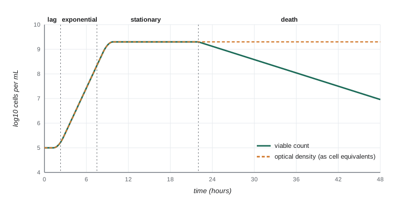
Stationary phase is not a period of inactivity. When nutrients run out, bacteria activate the stringent response, in which the alarmone (p)ppGpp shuts down ribosome synthesis and redirects resources to amino acid synthesis and stress survival. In E. coli, the sigma factor RpoS switches on genes that protect against oxidative stress, heat and acid, so stationary-phase cells are far hardier than exponential cells, which matters when testing disinfectants and food processes. Cells also communicate their density by quorum sensing (lesson 10), and many antibiotic-producing species start making antibiotics only as growth slows.
The shape of the growth curve can be captured by a simple model that ties growth rate to substrate concentration. Jacques Monod showed in the 1940s that the specific growth rate depends on the concentration S of the limiting substrate in a saturating way:
Here μ_max is the maximum specific growth rate and K_s is the half-saturation constant, the substrate concentration at which μ is half its maximum. The equation has the same form as Michaelis–Menten enzyme kinetics, although it describes whole cells. Values of K_s for sugars are often in the micromolar range, so cells grow at nearly full speed until the substrate is almost gone, which is why the transition from exponential to stationary phase is abrupt. If biomass X is produced with a constant yield Y (grams of cells per gram of substrate consumed), then dX/dt = μX and dS/dt = −μX/Y, and the final biomass is approximately X₀ + YS₀.
import numpy as np
from scipy.integrate import solve_ivp

mu_max, Ks, Y = 1.0, 0.05, 0.5            # per h, g/L, g cells per g glucose
S0, X0 = 2.0, 0.002                       # g/L
def rhs(t, z):
    X, S = z
    S = max(S, 0.0)
    mu = mu_max * S / (Ks + S)
    return [mu * X, -mu * X / Y]
sol = solve_ivp(rhs, (0, 12), [X0, S0], t_eval=np.arange(0, 12.5, 1.0), rtol=1e-8, atol=1e-10)
print(" t(h)   X (g/L)   S (g/L)   mu (per h)")
for t, X, S in zip(sol.t, sol.y[0], sol.y[1]):
    S = max(S, 0.0)
    print(f"{t:4.0f}  {X:8.4f}  {S:8.4f}  {mu_max*S/(Ks+S):8.3f}")
print(f"predicted final biomass X0 + Y*S0 = {X0 + Y*S0:.3f} g/L")t(h) X (g/L) S (g/L) mu (per h) 0 0.0020 2.0000 0.976 1 0.0053 1.9934 0.976 2 0.0141 1.9759 0.975 3 0.0373 1.9294 0.975 4 0.0988 1.8064 0.973 5 0.2609 1.4822 0.967 6 0.6783 0.6473 0.928 7 1.0020 0.0000 0.000 8 1.0020 0.0000 0.000 9 1.0020 0.0000 0.000 10 1.0020 0.0000 0.000 11 1.0020 0.0000 0.000 12 1.0020 0.0000 0.000 predicted final biomass X0 + Y*S0 = 1.002 g/L
The model has no lag phase, but it reproduces the rest of the curve: μ stays near μ_max while glucose is abundant, the biomass rises exponentially, and in the last hour the glucose collapses and growth stops within a single doubling, leaving close to Y × S₀ = 1 g of cells per litre. Real cultures also show diauxie when two sugars are present: E. coli grows first on glucose and then, after a pause, on lactose, because glucose represses the lac operon (BIOL-207). Each sugar produces its own exponential phase.
Continuous culture and the chemostat
A batch culture passes through its phases and cannot be held at one of them. A chemostat solves this. Fresh medium with a growth-limiting nutrient at concentration S_R flows into a stirred vessel of volume V at a flow rate F, and culture flows out at the same rate, keeping the volume constant. The dilution rate is D = F/V, the fraction of the vessel volume replaced per hour. Cells are washed out at rate DX, so the biomass changes as dX/dt = (μ − D)X. A steady state is reached when growth exactly balances washout, which means μ = D. The experimenter therefore sets the growth rate simply by setting the pump. Substituting the Monod equation gives the steady-state substrate concentration and biomass:
These equations make two predictions. The steady-state substrate concentration depends only on D and the organism’s growth parameters, not on the concentration in the feed, so a chemostat holds the limiting nutrient at a very low, constant level. And if D approaches μ_max, S* rises towards S_R, X* falls towards zero and the culture washes out, because the cells cannot divide fast enough to replace those lost in the outflow.
import numpy as np

mu_max, Ks, Y, SR = 1.0, 0.05, 0.5, 2.0
print("  D (per h)   S* (g/L)   X* (g/L)   productivity D*X* (g/L/h)")
for D in [0.1, 0.3, 0.5, 0.7, 0.9, 0.95, 0.97]:
    S = Ks * D / (mu_max - D)
    X = max(Y * (SR - S), 0.0)
    print(f"  {D:8.2f}  {S:9.4f}  {X:9.4f}  {D*X:10.4f}")
Dc = mu_max * SR / (Ks + SR)
print(f"critical (washout) dilution rate = {Dc:.3f} per h")
Dopt = mu_max * (1 - np.sqrt(Ks / (Ks + SR)))
print(f"dilution rate giving maximum productivity = {Dopt:.3f} per h") D (per h) S* (g/L) X* (g/L) productivity D*X* (g/L/h)
0.10 0.0056 0.9972 0.0997
0.30 0.0214 0.9893 0.2968
0.50 0.0500 0.9750 0.4875
0.70 0.1167 0.9417 0.6592
0.90 0.4500 0.7750 0.6975
0.95 0.9500 0.5250 0.4988
0.97 1.6167 0.1917 0.1859
critical (washout) dilution rate = 0.976 per h
dilution rate giving maximum productivity = 0.844 per h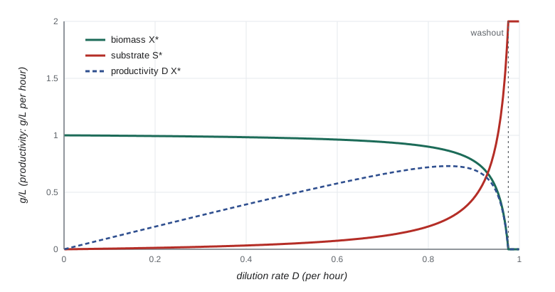
Chemostats are used to study physiology at controlled growth rates, to impose selection for particular traits in experimental evolution (BIOL-321), and in industry to make products continuously. Most industrial fermentations nevertheless use batch or fed-batch processes, in which nutrients are added gradually to a batch culture, because long continuous runs risk contamination and the selection of non-producing mutants that outgrow the producers. A related device, the turbidostat, adjusts the flow to hold the OD constant and keeps cells growing near μ_max.
Growth in nature
Laboratory cultures are a poor guide to microbial life outside the flask. In soils, sediments and the open ocean, nutrients are usually scarce and arrive in pulses, so most cells grow slowly or not at all for long periods. Many live attached to surfaces in biofilms, where gradients of oxygen and nutrients mean cells a few tens of micrometres apart experience completely different conditions. Microbial ecologists estimate in situ growth rates using methods such as the incorporation of labelled thymidine or leucine, the ratio of ribosomal RNA to DNA, and, from metagenomes, the peak-to-trough ratio of sequencing coverage across a genome, which is high in actively replicating populations. These methods confirm that doubling times of days to years are normal in nature.
Common mistakes
MistakeUsing natural logarithms in n = (log N − log N₀)/log 2 with base-10 logarithms elsewhere.
InsteadAny base works as long as numerator and denominator use the same one.
MistakeCounting a plate with 600 colonies because it is the only one available.
InsteadReport it as too numerous to count, or as an estimate with a warning; counts outside the countable range are unreliable.
MistakeReporting a viable count as cells per mL.
InsteadReport colony-forming units, because colonies may arise from clumps or chains.
MistakeAssuming optical density is proportional to cell number at any reading.
InsteadOD is linear only over a limited range and measures biomass; dilute dense samples and calibrate for the organism.
MistakeExpecting chemostat output to rise indefinitely with faster flow.
InsteadAbove the critical dilution rate the culture washes out; productivity peaks just below that point.
MistakeTreating stationary-phase cells as equivalent to exponential cells in disinfection tests.
InsteadStationary-phase cells switch on stress responses and are usually much more resistant.
Summary and key terms
- Binary fission gives N = N₀2ⁿ; the generation time is g = t/n, with n = (log N − log N₀)/log 2, and μ = ln 2/g.
- Total counts (microscopy, electronic counters, flow cytometry) include dead cells; viable counts measure colony-forming units on a chosen medium.
- Serial dilution brings samples into the countable range; CFU per mL = colonies/(volume plated × dilution).
- The most probable number method estimates low concentrations from the pattern of positive tubes using Poisson probabilities.
- Optical density tracks biomass and is linear only at low readings; growth rates are fitted to the exponential window of log OD.
- Batch cultures pass through lag, exponential, stationary and death phases; the Monod equation μ = μ_max S/(K_s + S) links growth to substrate.
- In a chemostat, μ = D at steady state; S* = K_s D/(μ_max − D), and the culture washes out as D approaches μ_max.
- binary fission
- Division of one cell into two similar daughter cells.
- generation time
- The time for a population to double in number during exponential growth.
- specific growth rate
- μ, the rate constant in dN/dt = μN, equal to ln 2 divided by the generation time.
- colony-forming unit
- A cell or group of cells that gives rise to one colony on a plate.
- serial dilution
- A series of stepwise dilutions, each multiplying the dilution of the previous one.
- most probable number
- A statistical estimate of concentration from the number of positive tubes in a dilution series.
- optical density
- A spectrophotometer measure of light scattering used to follow biomass.
- Monod equation
- μ = μ_max S/(K_s + S), relating specific growth rate to limiting substrate concentration.
- chemostat
- A continuous-culture vessel in which the dilution rate sets the growth rate at steady state.
- dilution rate
- D = F/V, the flow rate divided by the culture volume.
Practice problems
Work each problem on paper first, then reveal the answer to check.
A culture grows from 10³ to 10⁹ cells per mL in exponential phase. How many generations is that?
Show answer
log(10⁶)/log 2 = 6/0.301 ≈ 19.9 generations.
If that took 10 hours, what is the generation time?
Show answer
600/19.9 ≈ 30 minutes.
What is μ for a generation time of 30 minutes?
Show answer
ln 2/0.5 h ≈ 1.39 per hour.
A 10⁻⁶ dilution plated at 0.1 mL gives 156 colonies. What is the concentration?
Show answer
156/(0.1 × 10⁻⁶) = 1.56 × 10⁹ CFU per mL.
Three serial transfers of 0.5 mL into 4.5 mL are made. What is the final dilution?
Show answer
(1/10)³ = 10⁻³.
Why is an MPN confidence interval much wider than that of a plate count?
Show answer
It is based on presence or absence in a few tubes rather than on counts of many colonies.
An OD₆₀₀ reading is 1.2. What should you do before relying on it?
Show answer
Dilute the sample into the linear range (for example to an OD below about 0.4), measure and multiply by the dilution.
With μ_max = 0.8 per h and K_s = 0.1 g/L, what is μ at S = 0.1 g/L?
Show answer
Half of μ_max, 0.4 per hour.
A chemostat has V = 2 L and F = 0.6 L/h. What is the steady-state growth rate?
Show answer
D = 0.3 per hour, so μ = 0.3 per hour.
For the same organism (μ_max = 0.8, K_s = 0.1), what is S* at D = 0.4?
Show answer
S* = 0.1 × 0.4/(0.8 − 0.4) = 0.1 g/L.
Lesson quiz · 5 questions
Score 60% or more to complete this lesson.
Create a free account to save your progress, take quizzes and earn a certificate.