
BIOL-321 · Lesson 8 of 12 · 28 min
Phylogenetics I: building trees
A phylogeny is a hypothesis about the history of descent connecting a group of organisms. Phylogenies underpin almost every part of modern biology: they are used to classify organisms, trace the origin of pandemics, date evolutionary events and test hypotheses about adaptation. BIOL-108 introduced reading trees, UPGMA clustering and simple parsimony. This lesson builds the main methods of modern tree building: distance methods with corrections for multiple substitutions, neighbour-joining, parsimony scoring with the Fitch algorithm, the idea of maximum likelihood and Bayesian inference, and the bootstrap for measuring support.
Reading trees correctly
A rooted tree has a root representing the common ancestor of all included taxa; branches represent lineages and internal nodes represent ancestors at which lineages split. A clade, or monophyletic group, contains an ancestor and all its descendants. A paraphyletic group contains an ancestor and only some of its descendants, such as traditional reptiles, which exclude birds. A polyphyletic group lacks the common ancestor of its members, such as warm-blooded animals grouping birds and mammals. Trees can be rotated around any node without changing their meaning, so the left-to-right order of tips carries no information. Unrooted trees show relationships without specifying the direction of time; they are rooted by including an outgroup, a taxon known to lie outside the group of interest.
Two common errors are reading a tree as a ladder of progress, with one living species ancestral to another, and assuming that taxa next to each other on the page are closest relatives. Relatedness is measured by the recency of common ancestry: humans are more closely related to mushrooms than mushrooms are to plants, because animals and fungi share a more recent common ancestor.
The number of possible trees grows explosively with the number of taxa. For n taxa there are (2n − 5)!! unrooted bifurcating trees, where !! is the double factorial, the product of every second integer.
from math import prod
def n_unrooted(n):
    return prod(range(1, 2*n - 4, 2))   # (2n-5)!! = 1*3*5*...*(2n-5)
for n in (4, 5, 10, 20, 50):
print(f"{n:3d} taxa: {n_unrooted(n):.3e} unrooted trees")4 taxa: 3.000e+00 unrooted trees 5 taxa: 1.500e+01 unrooted trees 10 taxa: 2.027e+06 unrooted trees 20 taxa: 2.216e+20 unrooted trees 50 taxa: 2.838e+74 unrooted trees
With 20 taxa there are already more than 10^20 trees, so exhaustive search is impossible, and practical programs use heuristic searches that rearrange branches to improve a score, or algorithms such as neighbour-joining that build a single tree directly.
Distances and multiple hits
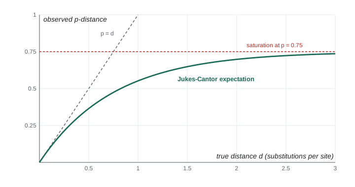
The simplest measure of divergence between two aligned DNA sequences is the p-distance, the proportion of sites that differ. But p underestimates the true number of substitutions, because a site can change more than once (A to G and back, or A to G to T), and later changes hide earlier ones. These are called multiple hits, and they become important as sequences diverge. The Jukes–Cantor (1969) model assumes all four bases are equally frequent and every substitution equally likely. Under this model, the expected number of substitutions per site d is
As p approaches 0.75, the value expected for two random sequences, d goes to infinity: the sequences are saturated and no longer contain information about how far apart they are. More realistic models, such as Kimura’s two-parameter model, which distinguishes transitions (purine to purine, pyrimidine to pyrimidine) from transversions, and the general time-reversible (GTR) model, with gamma-distributed rate variation among sites, are standard in practice.
import numpy as np
rng = np.random.default_rng(321)
L = 2000
bases = np.array(list("ACGT"))
def evolve(seq, d):
    """Jukes-Cantor evolution: each site gets Poisson(d*4/3) 'events', each replacing with a random base."""
    s = seq.copy()
    n_events = rng.poisson(d * 4/3, len(s))
    for i in np.nonzero(n_events)[0]:
        for _ in range(n_events[i]):
            s[i] = rng.integers(4)
    return s
anc = rng.integers(4, size=L)
print(" true d   observed p   JC estimate")
for d in (0.05, 0.2, 0.5, 1.0, 2.0):
    a, b = evolve(anc, d/2), evolve(anc, d/2)
    p = np.mean(a != b)
    jc = -0.75*np.log(1 - 4*p/3) if p < 0.75 else float("inf")
print(f"{d:6.2f} {p:9.3f} {jc:10.3f}")true d observed p JC estimate 0.05 0.045 0.046 0.20 0.172 0.196 0.50 0.372 0.515 1.00 0.563 1.042 2.00 0.681 1.795
For small distances p and d are nearly equal, but at a true distance of two substitutions per site, the observed proportion of differences is close to saturation, and only the correction gives a sensible estimate, with growing uncertainty. This is why rapidly evolving sites, such as third codon positions, are less useful for deep divergences.
Neighbour-joining
UPGMA assumes a molecular clock, so that all tips are equally distant from the root; when rates differ among lineages, UPGMA can give the wrong tree. Neighbour-joining, introduced by Naruya Saitou and Masatoshi Nei in 1987, does not assume a clock. At each step it chooses the pair of taxa i and j that minimizes
which corrects the raw distance by how far each taxon is from all others. A taxon on a long branch is far from everything, and subtracting its total distance prevents it from being joined incorrectly. The chosen pair is joined to a new node, branch lengths are calculated, distances from the new node to the remaining taxa are computed and the process repeats until three nodes remain.
import numpy as np
def nj_tree(D, names):
    D = D.astype(float).copy(); names = list(names); edges = []
    while len(names) > 2:
        n = len(names); r = D.sum(axis=1)
        Q = (n - 2) * D - r[:, None] - r[None, :]
        np.fill_diagonal(Q, np.inf)
        i, j = np.unravel_index(np.argmin(Q), Q.shape)
        li = 0.5 * D[i, j] + (r[i] - r[j]) / (2 * (n - 2))
        lj = D[i, j] - li
        new = f"({names[i]}:{li:.2f},{names[j]}:{lj:.2f})"
        dnew = 0.5 * (D[i] + D[j] - D[i, j])
        keep = [k for k in range(n) if k not in (i, j)]
        D = np.vstack([np.column_stack([D[np.ix_(keep, keep)], dnew[keep]]),
                       np.append(dnew[keep], 0.0)])
        names = [names[k] for k in keep] + [new]
    return f"({names[0]}:{D[0,1]:.2f},{names[1]});"

# Additive distances from a tree with unequal rates: A and B are sisters, but B evolves fast
names = ["A", "B", "C", "D"]
D = np.array([[0, 7, 4, 6],
              [7, 0, 9, 11],
              [4, 9, 0, 4],
              [6, 11, 4, 0]])
print("NJ tree:", nj_tree(D, names))
# UPGMA would first join the closest pair (A,C or C,D at distance 4), not the true sisters A and BNJ tree: ((A:1.00,B:6.00):2.00,(C:1.00,D:3.00));
These distances are additive: they come from a tree in which A and B are sisters, but B has a long branch because it evolves rapidly. The smallest raw distance (4) links A with C and C with D, so a method that simply joins the closest pair would group A and C. The Q criterion corrects for B being far from everything and recovers the true pairing of A and B, with B on a branch of length 6, A on a branch of length 1 and an internal branch of length 2 separating the pair AB from the pair CD. Neighbour-joining is fast, works for thousands of sequences and is statistically consistent when distances are estimated well, but it gives a single tree with no measure of how strongly the data support it.
Parsimony and the Fitch algorithm
Maximum parsimony chooses the tree that requires the fewest changes to explain the observed characters. For a given tree, Walter Fitch’s 1971 algorithm counts the minimum number of changes at each site by moving from tips to root: at each internal node, if the sets of states of its two children overlap, take the intersection; if not, take the union and add one change.
Worked problem
Fitch parsimony at one site
Four taxa have bases A: G, B: G, C: T, D: A at one site. Count the minimum changes on tree ((A,B),(C,D)) and on tree ((A,C),(B,D)).
Show solution
- Tree ((A,B),(C,D)): node AB = {G} ∩ {G} = {G}, no change. Node CD = {T} ∪ {A} = {A, T}, one change. Root: {G} and {A, T} do not overlap, union, one more change. Total 2.
- Tree ((A,C),(B,D)): node AC = {G, T}, one change. Node BD = {G, A}, one change. Root: {G, T} ∩ {G, A} = {G}, no change. Total 2.
- Both trees need two changes, so this site does not distinguish them. Only sites with at least two states each present in at least two taxa (parsimony-informative sites) can favour one tree over another.
Answer: Two changes on each tree; the site is uninformative for choosing between them.
Parsimony is intuitive and makes few explicit assumptions, but those assumptions can be violated. Joseph Felsenstein showed in 1978 that when two unrelated lineages have long branches, parsimony tends to group them together, because they accumulate many parallel changes by chance. This long-branch attraction makes parsimony statistically inconsistent in some situations: adding more data makes it more confident in the wrong tree. Model-based methods correct for multiple hits and are less affected.
Maximum likelihood and Bayesian inference
Maximum likelihood, made practical for DNA by Felsenstein in 1981, asks which tree and branch lengths make the observed data most probable under an explicit model of substitution. For one site on a given tree, the likelihood is the sum over all possible states at the internal nodes of the probability of the observed tip states; Felsenstein’s pruning algorithm computes this efficiently. The likelihood for the whole alignment is the product over sites, or the sum of log-likelihoods. Programs such as RAxML-NG and IQ-TREE search tree space for the highest likelihood and also choose among substitution models using criteria such as AIC or BIC.
Under the Jukes–Cantor model, the probability that a site is the same at the two ends of a branch of length t (in expected substitutions per site) is
and the probability that it changes to one particular other base is one-third of the remainder. For two sequences differing at k of n sites, the likelihood is maximized at the Jukes–Cantor distance, as the next code confirms by brute force.
import numpy as np
n, k = 500, 120            # sites compared, sites that differ (invented)
t = np.linspace(0.01, 1.0, 10000)
p_same = 0.25 + 0.75*np.exp(-4*t/3)
p_diff = (1 - p_same)      # probability of any difference (3 equally likely other bases)
loglik = (n - k)*np.log(p_same) + k*np.log(p_diff/3)
t_ml = t[np.argmax(loglik)]
p = k/n
print(f"p-distance = {p:.3f}")
print(f"maximum-likelihood distance = {t_ml:.4f}")
print(f"Jukes-Cantor formula = {-0.75*np.log(1 - 4*p/3):.4f}")p-distance = 0.240 maximum-likelihood distance = 0.2892 Jukes-Cantor formula = 0.2892
Bayesian phylogenetics, implemented in programs such as MrBayes, BEAST and RevBayes, combines the likelihood with prior distributions on trees, branch lengths and model parameters to give a posterior distribution, sampled by Markov chain Monte Carlo. The output is a set of trees, and the posterior probability of a clade is the proportion of sampled trees that contain it. Bayesian methods integrate over uncertainty in parameters and are especially convenient for dating (Lesson 9).
| Method | Optimality criterion | Strengths | Weaknesses |
|---|---|---|---|
| UPGMA | Clustering by average distance | Very fast; gives an ultrametric tree | Assumes a clock; wrong when rates vary |
| Neighbour-joining | Minimum evolution approximated by Q | Fast, no clock assumption, scales to many taxa | Single tree; depends on distance estimates |
| Maximum parsimony | Fewest changes | Simple; works for morphology | Long-branch attraction; no model of change |
| Maximum likelihood | Highest probability of data given tree and model | Explicit model; statistically consistent if model is adequate | Computationally heavy; model choice matters |
| Bayesian | Posterior probability | Measures uncertainty; flexible models with priors | Priors influence results; needs convergence checks |
Measuring support: the bootstrap
How confident should we be in a clade? Felsenstein introduced the nonparametric bootstrap to phylogenetics in 1985. The alignment columns are resampled with replacement to create many pseudo-alignments of the same length; a tree is built from each; and the bootstrap support for a clade is the percentage of replicate trees that contain it. Values above about 70 % are often considered reasonable support, but bootstrap values are not probabilities that the clade is true, and with genome-scale data almost every clade receives 100 %, even when different genes tell different stories.
import numpy as np
rng = np.random.default_rng(321)
# Four taxa, 300 sites. Each site is invented as supporting split AB|CD, AC|BD or AD|BC, or uninformative.
L = 300
site_type = rng.choice(["AB", "AC", "AD", "none"], size=L, p=[0.10, 0.06, 0.05, 0.79])
def best_split(cols):
    counts = {s: np.sum(cols == s) for s in ("AB", "AC", "AD")}
    return max(counts, key=counts.get)
print("original data support:", best_split(site_type),
      {s: int(np.sum(site_type == s)) for s in ("AB", "AC", "AD")})
B = 1000
wins = {"AB": 0, "AC": 0, "AD": 0}
for _ in range(B):
    wins[best_split(rng.choice(site_type, size=L, replace=True))] += 1
for s, w in wins.items():
print(f"bootstrap support for {s}|rest: {100*w/B:5.1f} %")original data support: AB {'AB': 25, 'AC': 20, 'AD': 18}
bootstrap support for AB|rest: 71.6 %
bootstrap support for AC|rest: 19.8 %
bootstrap support for AD|rest: 8.6 %Here the split grouping A with B has the most informative sites, and the bootstrap shows how often resampling the data would still favour it. When the signal is weak, as in rapid radiations where lineages split in quick succession, bootstrap support is low and different genes may support different trees, because ancestral polymorphisms sort randomly into descendant lineages, a process called incomplete lineage sorting. Coalescent-based species tree methods, introduced in BIOL-322, address this problem, and genome-scale phylogenomics is covered in BIOL-410.
Common mistakes
MistakeTaxa next to each other at the tips are closest relatives.
InsteadRelatedness is shown by branching order; rotating nodes changes tip order without changing relationships.
MistakeA living species can be the ancestor of another living species on a tree.
InsteadLiving species are all tips; their common ancestors are internal nodes.
MistakeThe p-distance measures the number of substitutions.
InsteadIt underestimates them because of multiple hits; correct with a model such as Jukes–Cantor.
MistakeParsimony is always reliable because it makes no assumptions.
InsteadParsimony is inconsistent under long-branch attraction; its implicit assumptions can fail.
MistakeA bootstrap value of 90 % means a 90 % chance the clade is real.
InsteadIt measures how consistently the data support the clade when resampled, not the probability of truth.
MistakeGene trees always match the species tree.
InsteadIncomplete lineage sorting and hybridization make gene trees differ from species trees.
Summary and key terms
- Clades are monophyletic; tip order carries no information; outgroups root unrooted trees.
- The number of possible trees grows as (2n − 5)!!, so heuristic search or direct algorithms are needed.
- Observed differences saturate; the Jukes–Cantor correction d = −(3/4) ln(1 − 4p/3) estimates substitutions per site.
- Neighbour-joining uses the Q criterion to join pairs without assuming a clock.
- Fitch’s algorithm counts parsimony changes; long-branch attraction can mislead parsimony.
- Maximum likelihood and Bayesian inference use explicit models; the ML distance between two sequences equals the Jukes–Cantor distance.
- Bootstrap resampling of sites measures support, which is not the same as the probability that a clade is correct.
- clade
- An ancestor and all of its descendants; a monophyletic group.
- paraphyletic
- Including an ancestor but not all of its descendants.
- outgroup
- A taxon outside the group of interest, used to root a tree.
- multiple hits
- Repeated substitutions at the same site that hide earlier changes.
- Jukes–Cantor model
- A substitution model with equal base frequencies and equal rates of change.
- neighbour-joining
- A distance method that joins pairs minimizing the Q criterion.
- maximum parsimony
- Choosing the tree that requires the fewest character changes.
- long-branch attraction
- The tendency of methods, especially parsimony, to group long branches incorrectly.
- maximum likelihood
- Choosing the tree and parameters that make the data most probable under a model.
- bootstrap
- Resampling alignment columns with replacement to assess clade support.
Practice problems
Work each problem on paper first, then reveal the answer to check.
How many unrooted trees are there for 6 taxa?
Show answer
(2 × 6 − 5)!! = 7!! = 1 × 3 × 5 × 7 = 105.
Is "fish" a monophyletic group? Explain.
Show answer
No; the common ancestor of fish is also the ancestor of tetrapods, so fish is paraphyletic.
Calculate the Jukes–Cantor distance for p = 0.30.
Show answer
d = −0.75 ln(1 − 0.4) = −0.75 ln 0.6 ≈ 0.383.
What happens to the JC distance as p approaches 0.75?
Show answer
It goes to infinity: the sequences are saturated.
Why can UPGMA give the wrong tree when rates differ?
Show answer
It assumes a clock and joins the most similar pair, which may not be sisters if one lineage evolves faster.
What does the Q criterion correct for?
Show answer
How far each taxon is from all others, so long branches are not mistakenly joined.
What is a parsimony-informative site?
Show answer
A site with at least two states each present in at least two taxa.
Describe long-branch attraction.
Show answer
Two long branches accumulate many chance parallel changes and are grouped together incorrectly.
What is resampled in the nonparametric bootstrap?
Show answer
Alignment columns (sites), with replacement.
Why might a gene tree differ from the species tree?
Show answer
Incomplete lineage sorting, hybridization or gene duplication and loss.
Lesson quiz · 5 questions
Score 60% or more to complete this lesson.
Create a free account to save your progress, take quizzes and earn a certificate.