Natural selection and adaptation in depth

Natural selection is simple to state and surprisingly subtle to apply. BIOL-108 showed how a favoured allele spreads in a population, and BIOL-201 showed how selection against a recessive allele slows as the allele becomes rare. This lesson builds the theory more carefully. It defines fitness precisely, distinguishes the modes of selection on traits, shows how selection can maintain variation as well as remove it, and asks what adaptation really means and what limits it. Throughout, the aim is to move from words to numbers: selection is a measurable force, and its consequences can be predicted.

What fitness means

In evolutionary biology, fitness is not strength or health but reproductive success: the average contribution of a genotype or phenotype to the next generation. Absolute fitness, W, is the expected number of offspring an individual leaves, counting survival and reproduction together. Relative fitness, w, is absolute fitness divided by that of a reference type, usually the fittest or the mean. Only relative fitness matters for changes in frequency, because a population of uniformly fit individuals does not change in composition however many offspring each leaves.

The selection coefficient, s, measures how much worse a type does than the reference: w = 1 − s. A selection coefficient of 0.01 means a 1 per cent disadvantage per generation. This may seem tiny, but over thousands of generations it is decisive. Fitness has components, such as viability (surviving to reproduce), fecundity (number of offspring), mating success and generation time, and selection can act differently on each.

Selection at one locus: dominance matters

For a diploid locus with alleles A and a at frequencies p and q, the change in frequency each generation depends on the fitnesses of the three genotypes. A useful general form is Δq = pq[q(w_aa − w_Aa) + p(w_Aa − w_AA)] / w̄, where w̄ is the mean fitness. Two features follow. First, change is proportional to pq, so selection is weak when either allele is rare. Second, dominance determines where selection is effective. A favourable dominant allele spreads quickly at first, because heterozygotes already benefit, but is slow to eliminate the last recessive copies. A favourable recessive allele spreads slowly at first, because it is hidden in heterozygotes, then rapidly once homozygotes are common. This asymmetry explains why harmful recessive alleles persist for so long in human populations (BIOL-201).

import numpy as np

def trajectory(h, s=0.05, p0=0.01, gens=4000):
    """Frequency of beneficial allele A; fitnesses AA = 1+s, Aa = 1+h*s, aa = 1."""
    p = p0; out = []
    for t in range(gens):
        q = 1 - p
        w = np.array([1 + s, 1 + h*s, 1.0])
        g = np.array([p*p, 2*p*q, q*q])
        wbar = (g*w).sum()
        p = (g[0]*w[0] + 0.5*g[1]*w[1]) / wbar
        out.append(p)
    return np.array(out)

def first(tr, x):
    hit = np.nonzero(tr > x)[0]
    return int(hit[0]) + 1 if hit.size else None

for h, name in [(1.0, "dominant"), (0.5, "additive"), (0.0, "recessive")]:
    tr = trajectory(h)
    t10, t99 = first(tr, 0.10), first(tr, 0.99)
    print(f"{name:9s}: 1% to 10% in {t10:4d} gens; 10% to 99% in {t99 - t10:4d} gens")

dominant : 1% to 10% in   52 gens; 10% to 99% in 2213 gens
additive : 1% to 10% in   98 gens; 10% to 99% in  279 gens
recessive: 1% to 10% in 1851 gens; 10% to 99% in  320 gens

The dominant allele leaves rarity quickly but crawls at the end; the recessive allele is stuck near rarity for a long time and then accelerates. The additive case, in which each copy adds the same amount, is in between and is the usual default in theory. In large populations, a new beneficial mutation that is recessive faces an additional problem: while rare, it is almost always in heterozygotes and invisible to selection, so drift may lose it before selection can act. This is called Haldane’s sieve, and it means that adaptations from new mutations tend to involve dominant or additive alleles.

Modes of selection on a trait

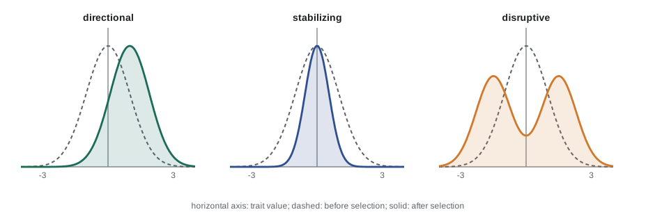
Many traits, such as body size, beak depth or flowering time, vary continuously. Selection on such a trait can be described by how fitness changes across the range of phenotypes. Under directional selection, fitness increases steadily toward one extreme, and the mean shifts in that direction. Under stabilizing selection, intermediate phenotypes have the highest fitness, so the mean stays put and variance shrinks. Under disruptive selection, both extremes do better than the middle, which can increase variance and, in some circumstances, contribute to speciation (lesson 7). Human birth weight was a classic example of stabilizing selection: in mid-twentieth-century data, infants near 3.5 kg had the highest survival, although modern medical care has weakened this selection.

import numpy as np
rng = np.random.default_rng(321)
z = rng.normal(10.0, 1.0, 100_000)            # trait values before selection (e.g. beak depth, mm)

fitness = {
    "directional": np.exp(0.5*(z - 10)),                # larger is better
    "stabilizing": np.exp(-(z - 10)**2 / (2*0.8**2)),   # optimum at 10
    "disruptive":  1 - 0.8*np.exp(-(z - 10)**2 / (2*0.8**2)),
}
print(f"before: mean {z.mean():.2f}, SD {z.std():.2f}")
for mode, w in fitness.items():
    wn = w / w.mean()                                    # relative fitness
    mean_after = (wn*z).mean()
    sd_after = np.sqrt((wn*(z - mean_after)**2).mean())
    S = mean_after - z.mean()                            # selection differential
    print(f"{mode:11s}: mean {mean_after:.2f}, SD {sd_after:.2f}, selection differential S = {S:+.2f}")

before: mean 10.00, SD 1.00
directional: mean 10.50, SD 1.00, selection differential S = +0.50
stabilizing: mean 10.00, SD 0.62, selection differential S = +0.00
disruptive : mean 10.00, SD 1.27, selection differential S = -0.00

The selection differential, S, is the difference between the mean of the selected individuals, weighted by their fitness, and the mean of the whole population. Directional selection produces a large S; stabilizing and disruptive selection produce S near zero but change the variance in opposite directions. Lesson 5 shows how S translates into a response in the next generation through heritability, the breeder’s equation from BIOL-201, R = h²S.

Measuring selection in the wild

Russell Lande and Stevan Arnold showed in 1983 how to estimate selection from field data by regressing relative fitness on traits. The slope of the regression is the selection gradient, β, which measures how strongly selection acts directly on each trait, controlling for correlations with other traits. Adding a squared term gives the quadratic gradient, γ, which is negative under stabilizing selection and positive under disruptive selection. Reviews of hundreds of studies, beginning with Kingsolver and colleagues in 2001, found that directional selection in nature is usually modest, with a typical standardized gradient of about 0.15, and that strong stabilizing selection is less common than once assumed.

import numpy as np
rng = np.random.default_rng(3211)
n = 400
size = rng.normal(0, 1, n)                     # standardized body size
wing = 0.6*size + rng.normal(0, 0.8, n)        # wing length, correlated with size
wing = (wing - wing.mean())/wing.std()
# True selection: directly on size only (beta = 0.30), none on wing
fit = np.exp(0.30*size - 0.10*size**2 + rng.normal(0, 0.5, n))
w = fit / fit.mean()

# Univariate (total) selection on wing alone
b_wing_alone = np.polyfit(wing, w, 1)[0]
# Multiple regression: gradients controlling for the correlation
X = np.column_stack([np.ones(n), size, wing, size**2])
coef, *_ = np.linalg.lstsq(X, w, rcond=None)
print(f"selection on wing measured alone: {b_wing_alone:+.3f}")
print(f"gradients: beta(size) = {coef[1]:+.3f}, beta(wing) = {coef[2]:+.3f}, "
      f"gamma(size) = {2*coef[3]:+.3f}")

selection on wing measured alone: +0.211
gradients: beta(size) = +0.246, beta(wing) = +0.054, gamma(size) = -0.074

Measured alone, wing length appears to be under positive selection, but only because long-winged birds also tend to be large. Multiple regression shows that selection acts mainly on size: the wing gradient is small, about a quarter of the size gradient, and much of the apparent selection on wings disappears. The negative quadratic term shows mild stabilizing selection on size. Distinguishing direct selection from correlated response is essential before claiming that a trait is adaptive.

Selection that maintains variation

Selection does not always remove variation. Several kinds of balancing selection keep two or more alleles in a population indefinitely. The best known is heterozygote advantage, or overdominance, in which heterozygotes are fitter than either homozygote. If the fitnesses are w_AA = 1 − s, w_AS = 1 and w_SS = 1 − t, the population reaches a stable equilibrium with the frequency of S equal to s/(s + t). The classic case is the sickle-cell allele of the β-globin gene in regions where Plasmodium falciparum malaria is common. Homozygotes for the normal allele are vulnerable to severe malaria, homozygotes for the sickle allele have sickle cell disease, and heterozygotes are substantially protected from malaria while having few symptoms.

In frequency-dependent selection, the fitness of a type depends on how common it is. Under negative frequency dependence, rare types do better, so no type can take over. Examples include self-incompatibility alleles in plants, which can only fertilize plants that do not share them, so rare alleles find more mates; host–parasite coevolution, in which parasites adapt to the commonest host genotype; and the left- and right-mouthed scale-eating cichlids of Lake Tanganyika, which attack prey from one side, so the rarer form surprises prey more often. Balancing selection also arises when selection varies in space or time, favouring different alleles in different habitats or years.

import numpy as np
# Negative frequency-dependent selection: fitness of type A falls as A becomes common
# w_A = 1 + 0.3*(0.5 - p), w_B = 1 + 0.3*(p - 0.5)   (illustrative)
for p0 in (0.05, 0.50, 0.90):
    p = p0
    for t in range(200):
        wA, wB = 1 + 0.3*(0.5 - p), 1 + 0.3*(p - 0.5)
        p = p*wA / (p*wA + (1 - p)*wB)
    print(f"start {p0:.2f} -> after 200 generations {p:.3f}")

start 0.05 -> after 200 generations 0.500
start 0.50 -> after 200 generations 0.500
start 0.90 -> after 200 generations 0.500

Whatever the starting frequency, the population converges on an equal mixture, the point where the two types have equal fitness. Balancing selection leaves a recognizable signature in DNA: unusually old alleles and high diversity around the selected site. The human leukocyte antigen (HLA) genes of the immune system are among the most diverse in the human genome, and some HLA allele lineages are older than the split between humans and chimpanzees, a sign of long-term balancing selection driven by pathogens.

Adaptation and its limits

An adaptation is a trait that evolved by natural selection because it improved fitness in a particular function. Not every useful trait is an adaptation for its current use. Feathers probably evolved first for insulation or display in dinosaurs and were later co-opted for flight. Stephen Jay Gould and Elisabeth Vrba called such traits exaptations. Some traits are not adaptations at all but by-products of other changes, or results of drift. Gould and Richard Lewontin warned in 1979 against the adaptationist programme of assuming every trait has an adaptive story, using the image of the spandrels of St Mark’s Basilica in Venice, the triangular spaces left over when arches meet a dome.

Adaptation is also limited. Selection can only act on variation that exists, so organisms are not perfectly designed. Trade-offs mean that improving one function costs another, as when larger eggs mean fewer eggs. Genetic correlations constrain how traits can change together (lesson 5). Phylogenetic history matters: the vertebrate eye has its photoreceptors behind a layer of nerves and blood vessels, creating a blind spot, while the independently evolved octopus eye does not. Environments change faster than populations can adapt, leaving organisms adapted to the past. Finally, selection maximizes fitness, not well-being or longevity: traits that help reproduction early in life can be favoured even if they cause harm later, an idea central to the evolutionary theory of ageing (lesson 12).

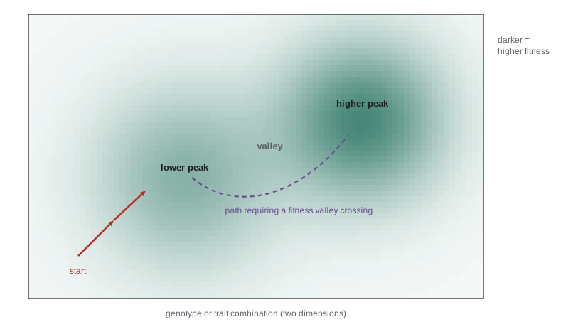
Sewall Wright pictured adaptation as populations climbing a fitness landscape, a surface relating genotype or phenotype to fitness. Selection always moves a population uphill, toward the nearest peak, even if a higher peak exists elsewhere, because getting there would mean crossing a valley of lower fitness. Wright suggested that drift in small, partly isolated populations might help populations cross valleys. Modern studies of real landscapes, made by measuring the fitness of every combination of a few mutations in a protein, find that many mutational paths to a better variant are blocked because intermediate steps are harmful, so evolution is often constrained to a few routes. Lesson 4 discusses why this kind of interaction among mutations, epistasis, makes evolution partly predictable and partly contingent.